第8章 · 原课件与完整中文翻译
上方为英文原页,下方为对应的完整中文翻译,标题、正文、图内文字和公式按原页顺序排列。
页号按PDF顺序。原课件的历史日期、学期、课堂安排和研究结论按原文保留;相关概念与适用条件见教程正文。符号、代码、作者姓名及便于检索的专有名称保留原文。
Lecture 08 · 105页
Lecture 08 · PDF p1
Lecture 08 · PDF p2
Lecture 08 · PDF p3
Lecture 08 · PDF p4
Lecture 08 · PDF p5
Lecture 08 · PDF p6
Lecture 08 · PDF p7
Lecture 08 · PDF p8
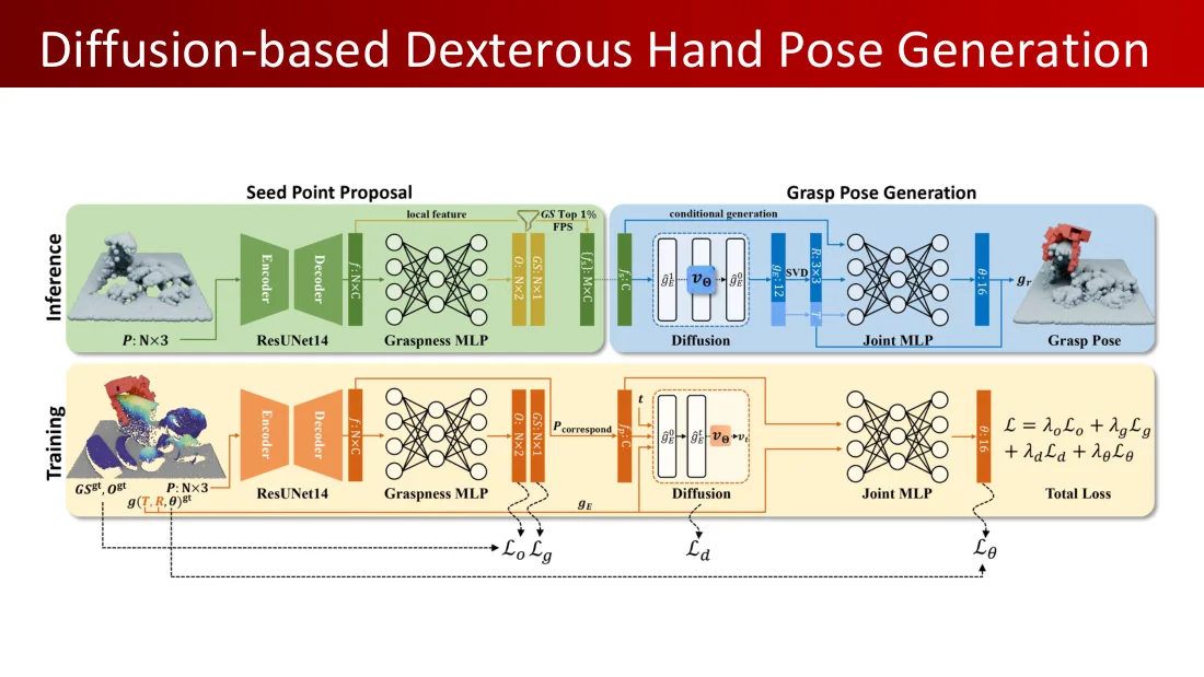
推理
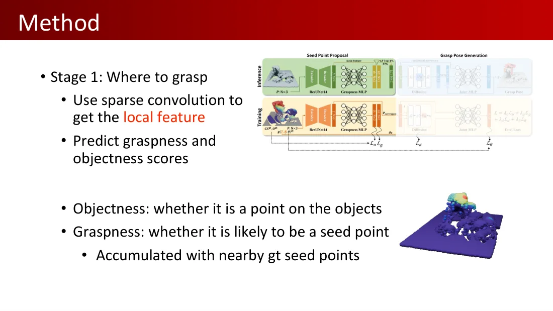
种子点提议:点云P(N×3)→ ResUNet14编码器 / 解码器 → 局部特征N×C → 可抓取性多层感知机 → 可抓取性GS(N×1)与物体性O(N×2);可抓取性前1%、最远点采样;种子特征f_s(M×C)。
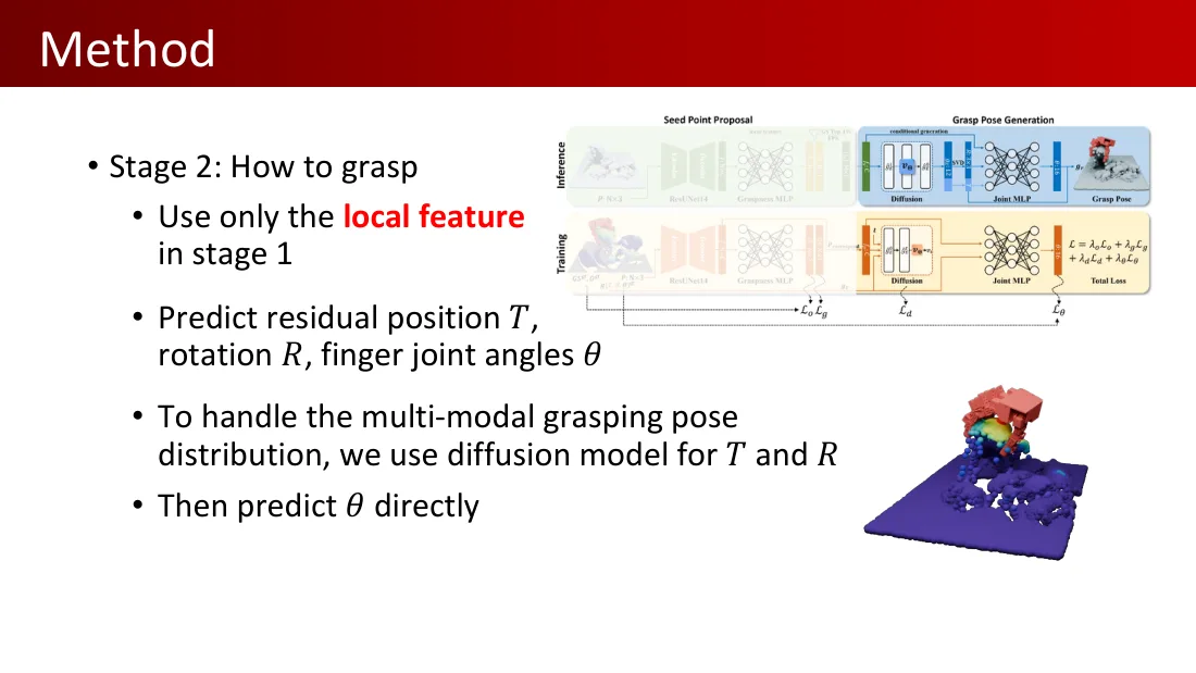
抓取位姿生成:条件生成;扩散;g_E¹ → v_θ → g_E⁰;GS_E:12维,R:3×3,奇异值分解SVD;关节多层感知机 → θ:16维 → 抓取位姿g_r。
训练
真值可抓取性GS^gt、物体性O^gt、抓取g(T,R,θ)^gt;点云P(N×3)→ ResUNet14编码器 / 解码器 → 可抓取性多层感知机;对应点P_correspond;扩散的时间t、g_Eᵗ、g_E⁰及预测v_θ和真值v_gt;关节多层感知机。
总损失:$L=\lambda_oL_o+\lambda_gL_g+\lambda_dL_d+\lambda_\theta L_\theta$。
Lecture 08 · PDF p9

阶段1:在哪里抓
- 使用稀疏卷积获得局部特征。
- 预测可抓取性与物体性分数。
- 物体性:是否为物体上的点。
- 可抓取性:是否可能成为种子点。
- 由邻近真值种子点累积得到。
推理
种子点提议:点云P(N×3)→ ResUNet14编码器 / 解码器 → 局部特征N×C → 可抓取性多层感知机 → 可抓取性GS(N×1)与物体性O(N×2);可抓取性前1%、最远点采样;种子特征f_s(M×C)。
抓取位姿生成:条件生成;扩散;g_E¹ → v_θ → g_E⁰;GS_E:12维,R:3×3,奇异值分解SVD;关节多层感知机 → θ:16维 → 抓取位姿g_r。
训练
真值可抓取性GS^gt、物体性O^gt、抓取g(T,R,θ)^gt;点云P(N×3)→ ResUNet14编码器 / 解码器 → 可抓取性多层感知机;对应点P_correspond;扩散的时间t、g_Eᵗ、g_E⁰及预测v_θ和真值v_gt;关节多层感知机。
总损失:$L=\lambda_oL_o+\lambda_gL_g+\lambda_dL_d+\lambda_\theta L_\theta$。
Lecture 08 · PDF p10

阶段2:怎样抓
- 仅使用阶段1的局部特征。
- 预测残差位置T、旋转R与手指关节角θ。
- 为处理多峰抓取位姿分布,使用扩散模型生成T和R。
- 随后直接预测θ。
推理
种子点提议:点云P(N×3)→ ResUNet14编码器 / 解码器 → 局部特征N×C → 可抓取性多层感知机 → 可抓取性GS(N×1)与物体性O(N×2);可抓取性前1%、最远点采样;种子特征f_s(M×C)。
抓取位姿生成:条件生成;扩散;g_E¹ → v_θ → g_E⁰;GS_E:12维,R:3×3,奇异值分解SVD;关节多层感知机 → θ:16维 → 抓取位姿g_r。
训练
真值可抓取性GS^gt、物体性O^gt、抓取g(T,R,θ)^gt;点云P(N×3)→ ResUNet14编码器 / 解码器 → 可抓取性多层感知机;对应点P_correspond;扩散的时间t、g_Eᵗ、g_E⁰及预测v_θ和真值v_gt;关节多层感知机。
总损失:$L=\lambda_oL_o+\lambda_gL_g+\lambda_dL_d+\lambda_\theta L_\theta$。
Lecture 08 · PDF p11
Lecture 08 · PDF p12
Lecture 08 · PDF p13
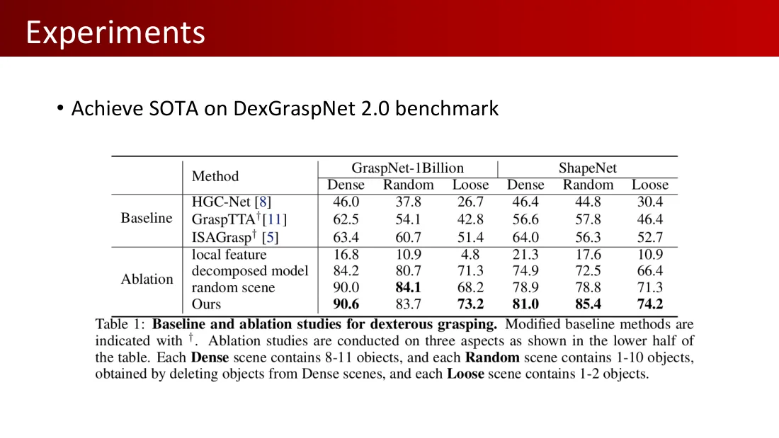
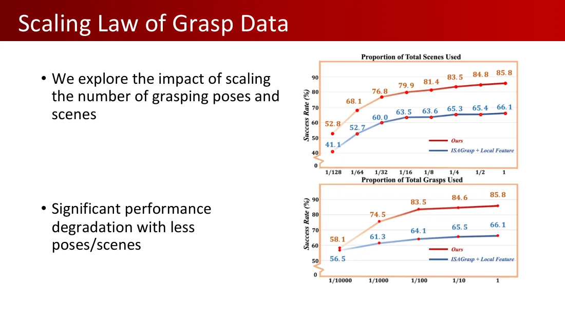
- 在DexGraspNet 2.0基准达到最先进水平。
| 组别 | 方法 | GraspNet密集 | GraspNet随机 | GraspNet疏松 | ShapeNet密集 | ShapeNet随机 | ShapeNet疏松 |
|---|---|---|---|---|---|---|---|
| 基线 | HGC-Net [8] | 46.0 | 37.8 | 26.7 | 46.4 | 44.8 | 30.4 |
| 基线 | GraspTTA† [11] | 62.5 | 54.1 | 42.8 | 56.6 | 57.8 | 46.4 |
| 基线 | ISAGrasp† [5] | 63.4 | 60.7 | 51.4 | 64.0 | 56.3 | 52.7 |
| 消融 | 局部特征 | 16.8 | 10.9 | 4.8 | 21.3 | 17.6 | 10.9 |
| 消融 | 分解模型 | 84.2 | 80.7 | 71.3 | 74.9 | 72.5 | 66.4 |
| 消融 | 随机场景 | 90.0 | 84.1 | 68.2 | 78.9 | 78.8 | 71.3 |
| 本文 | 本文方法 | 90.6 | 83.7 | 73.2 | 81.0 | 85.4 | 74.2 |
表1:灵巧抓取的基线与消融研究。†表示修改过的基线。消融研究围绕表格下半部分的三个方面进行。每个密集场景含8—11个物体;每个随机场景含1—10个物体,通过从密集场景删除物体获得;每个疏松场景含1—2个物体。
Lecture 08 · PDF p14
Lecture 08 · PDF p15
Lecture 08 · PDF p16
Lecture 08 · PDF p17
Lecture 08 · PDF p18
Lecture 08 · PDF p19
Lecture 08 · PDF p20
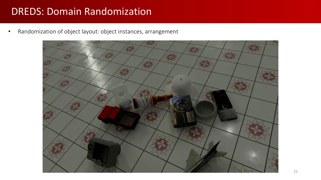
Lecture 08 · PDF p21
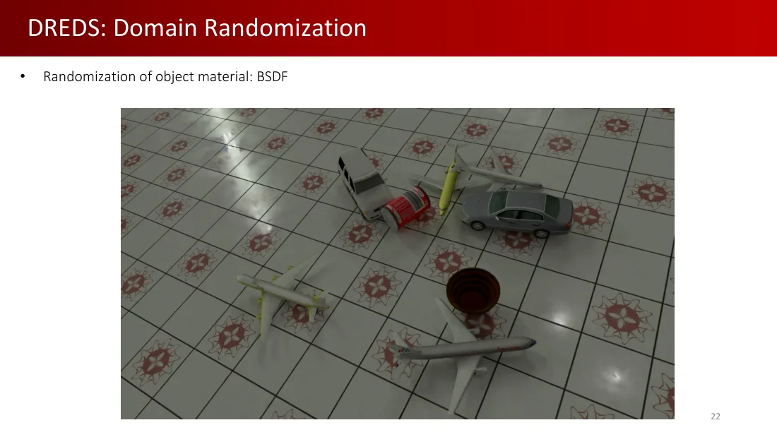
Lecture 08 · PDF p22
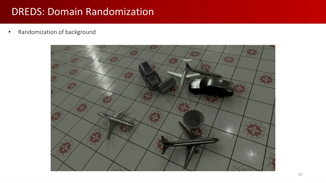
Lecture 08 · PDF p23
Lecture 08 · PDF p24
Lecture 08 · PDF p25
Lecture 08 · PDF p26
Lecture 08 · PDF p27
Lecture 08 · PDF p28
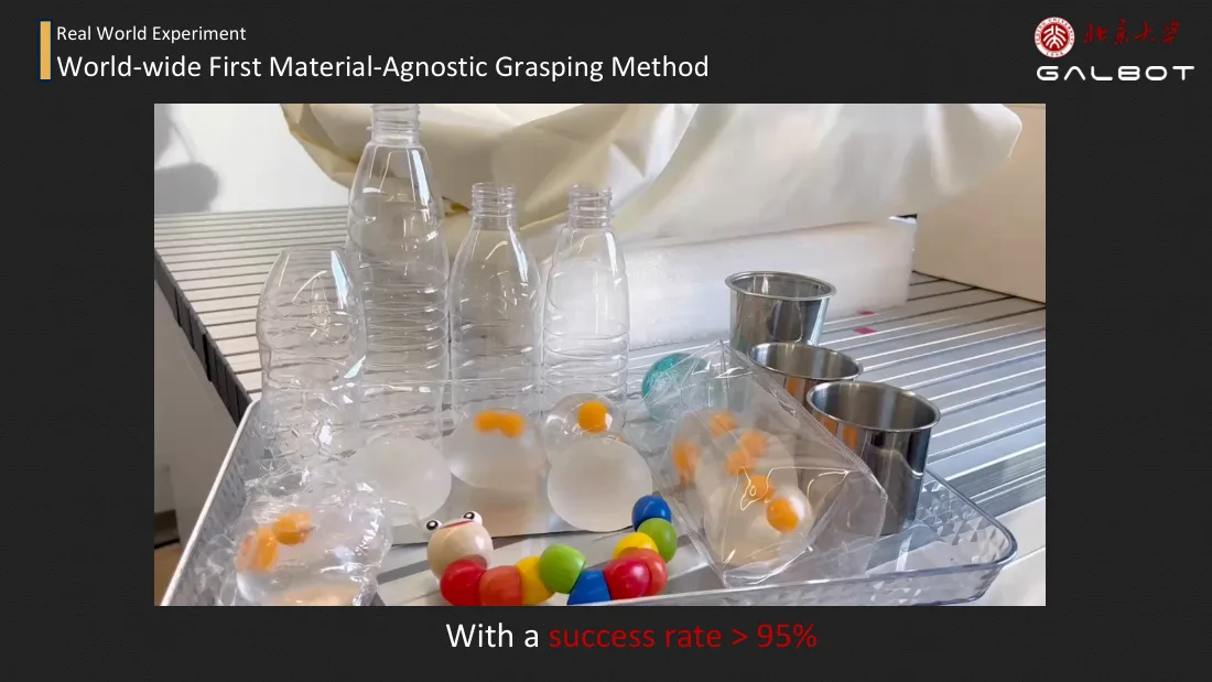
Lecture 08 · PDF p29
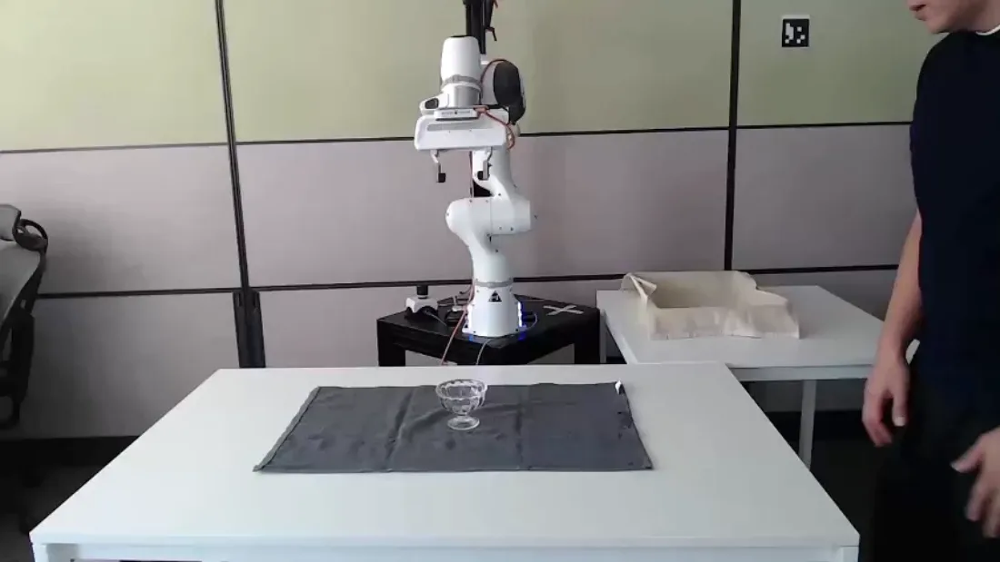
Lecture 08 · PDF p30
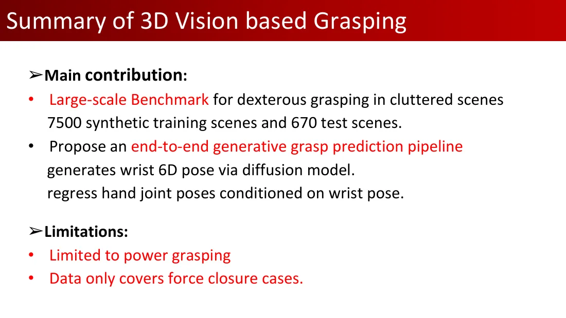
Lecture 08 · PDF p31
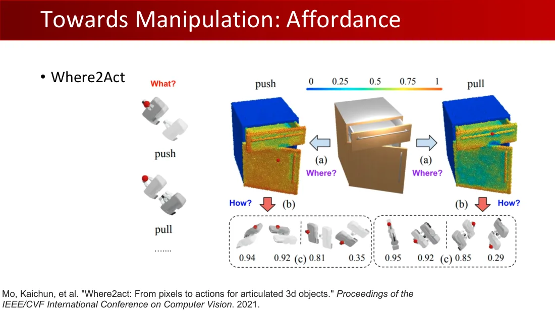
Lecture 08 · PDF p32
Lecture 08 · PDF p33
Lecture 08 · PDF p34
Lecture 08 · PDF p35
Lecture 08 · PDF p36
Lecture 08 · PDF p37
Lecture 08 · PDF p38
Lecture 08 · PDF p39
Lecture 08 · PDF p40
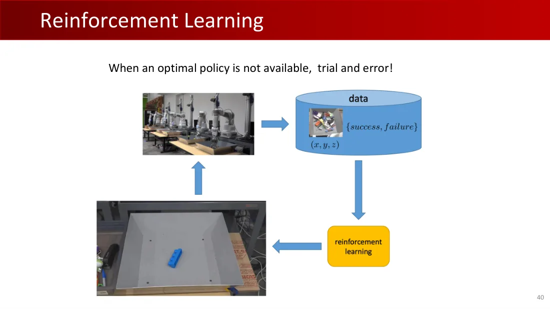
Lecture 08 · PDF p41
Lecture 08 · PDF p42
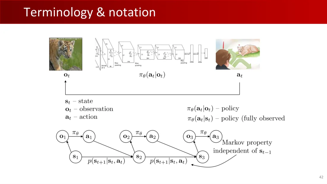
Lecture 08 · PDF p43
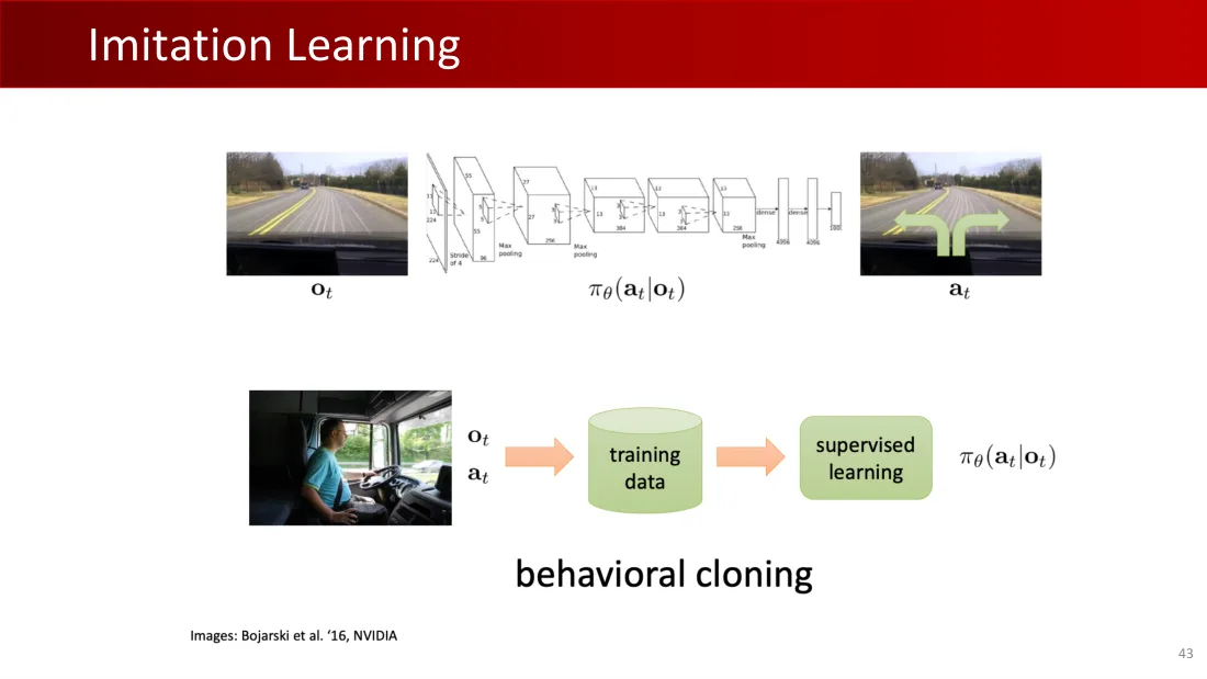
Lecture 08 · PDF p44
Lecture 08 · PDF p45
Lecture 08 · PDF p46
Lecture 08 · PDF p47
Lecture 08 · PDF p48
Lecture 08 · PDF p49
Lecture 08 · PDF p50
Lecture 08 · PDF p51
Lecture 08 · PDF p52
Lecture 08 · PDF p53
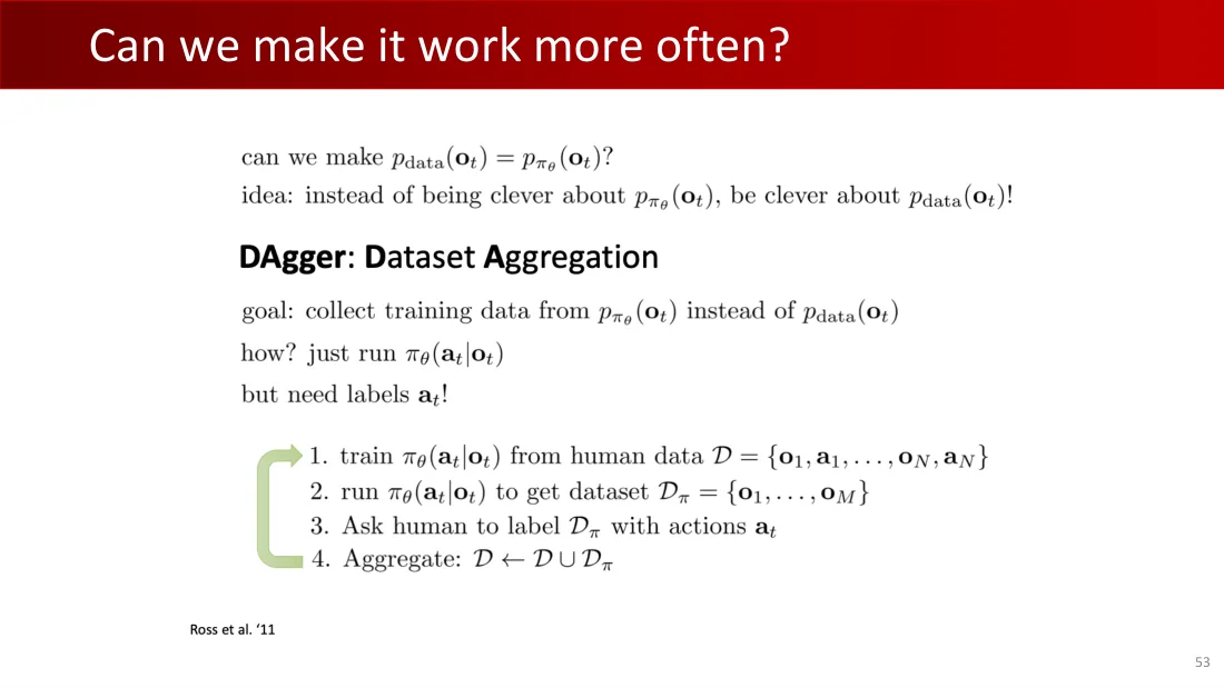
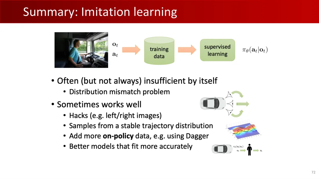
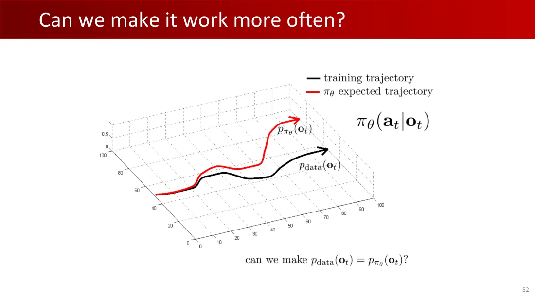
能否令$p_{data}(o_t)=p_{\pi_\theta}(o_t)$?
想法:与其巧妙处理p_πθ(oₜ),不如巧妙处理p_data(oₜ)!
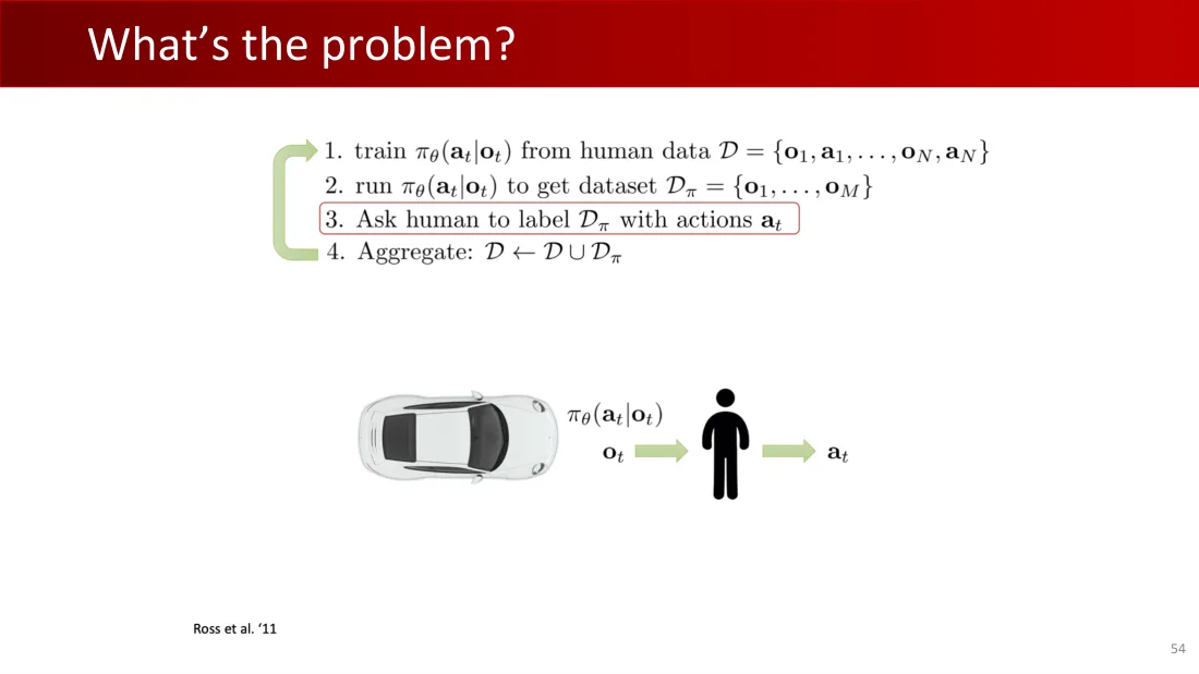
DAgger:数据集聚合
目标:从p_πθ(oₜ)而非p_data(oₜ)采集训练数据。
怎么做?直接执行πθ(aₜ|oₜ)。但还需要标签aₜ!
- 用人类数据$\mathcal D=\{o_1,a_1,\ldots,o_N,a_N\}$训练$\pi_\theta(a_t\mid o_t)$。
- 执行$\pi_\theta(a_t\mid o_t)$获得数据集$\mathcal D_\pi=\{o_1,\ldots,o_M\}$。
- 请人类为$\mathcal D_\pi$标注动作$a_t$。
- 聚合:$\mathcal D\leftarrow\mathcal D\cup\mathcal D_\pi$。
Ross等,2011。
Lecture 08 · PDF p54
Lecture 08 · PDF p55
Lecture 08 · PDF p56
Lecture 08 · PDF p57
Lecture 08 · PDF p58
Lecture 08 · PDF p59
Lecture 08 · PDF p60
Lecture 08 · PDF p61
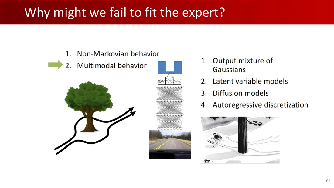
Lecture 08 · PDF p62
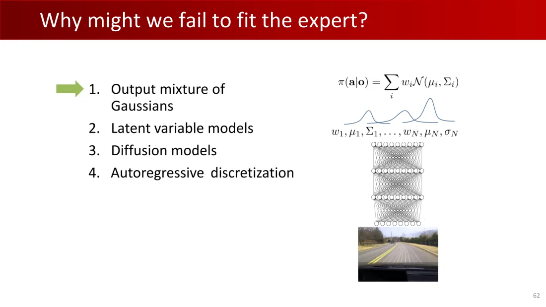
Lecture 08 · PDF p63
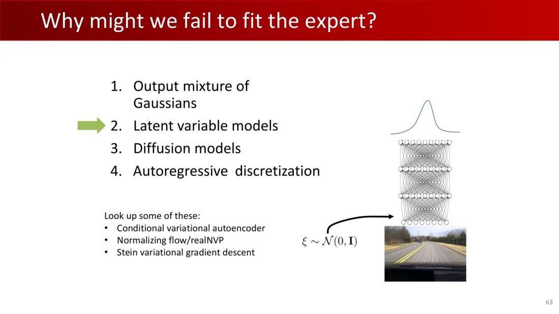
Lecture 08 · PDF p64
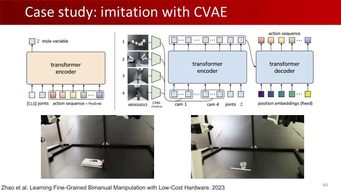
Lecture 08 · PDF p65
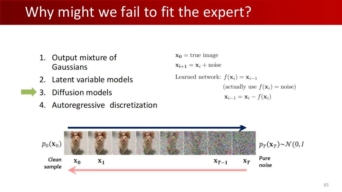
Lecture 08 · PDF p66
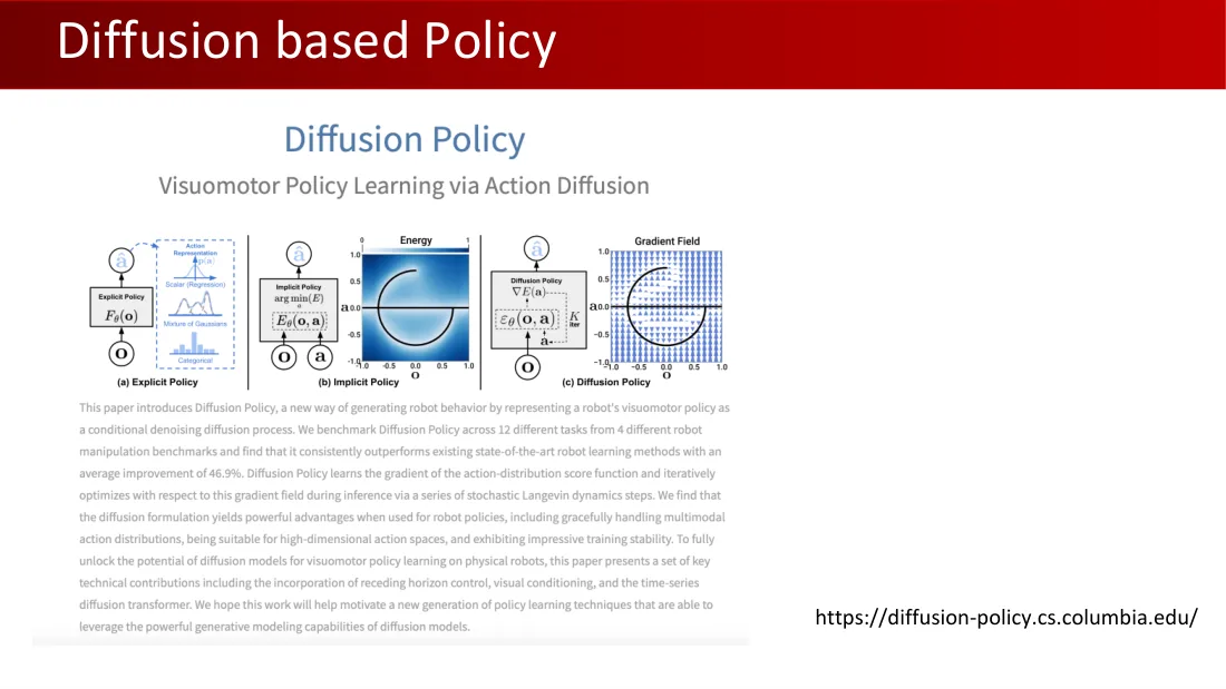
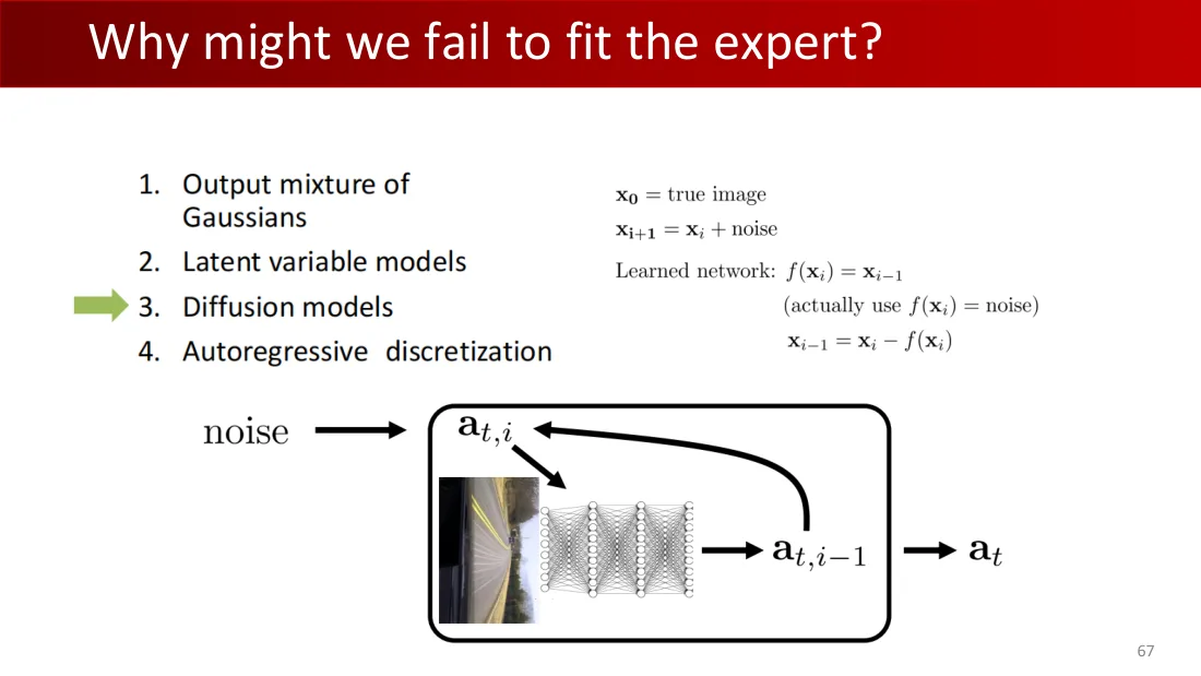
Diffusion Policy:扩散策略
通过动作扩散学习视觉运动策略。
(a)显式策略:$F_\theta(o)$;动作表示;标量(回归)、高斯混合、分类。
(b)隐式策略:$\arg\min(E)$,$E_\theta(o,a)$;能量;o、a。
(c)扩散策略:$\nabla E(a)$,$\epsilon_\theta(o,a)$;K次迭代;梯度场;o、a。
本文介绍扩散策略:一种通过条件去噪扩散过程表示机器人视觉运动策略、从而生成机器人行为的新方法。我们在4个机器人操作基准的12项不同任务上评测扩散策略,发现其持续优于现有最先进机器人学习方法,平均提升46.9%。扩散策略学习动作分布分数函数的梯度,并在推理时通过一系列随机朗之万动力学步骤沿此梯度场迭代优化。我们发现,扩散表述用于机器人策略时具有多项优势,包括平稳处理多峰动作分布、适合高维动作空间以及表现出良好训练稳定性。为充分释放扩散模型在实体机器人视觉运动策略学习中的潜力,本文提出一组关键技术贡献,包括引入滚动时域控制、视觉条件化以及时间序列扩散Transformer。我们希望这项工作推动新一代策略学习技术,利用扩散模型强大的生成建模能力。
https://diffusion-policy.cs.columbia.edu/
Lecture 08 · PDF p67
Lecture 08 · PDF p68
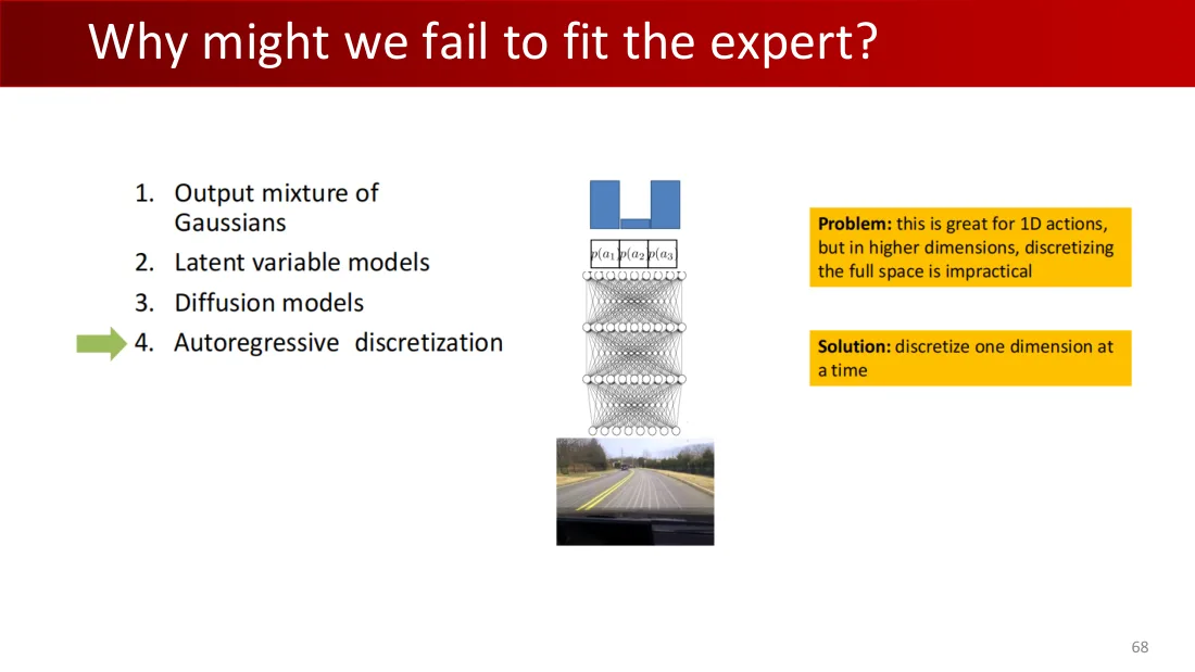
Lecture 08 · PDF p69
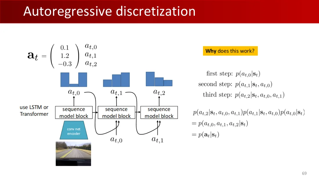
$a_t=(0.1,1.2,-0.3)^T$;分量$a_{t,0},a_{t,1},a_{t,2}$。
使用LSTM或Transformer;序列模型模块;共享视觉编码器。
为什么有效?
第一步:$p(a_{t,0}\mid s_t)$。第二步:$p(a_{t,1}\mid s_t,a_{t,0})$。第三步:$p(a_{t,2}\mid s_t,a_{t,0},a_{t,1})$。
$p(a_{t,2}\mid s_t,a_{t,0},a_{t,1})p(a_{t,1}\mid s_t,a_{t,0})p(a_{t,0}\mid s_t)=p(a_{t,0},a_{t,1},a_{t,2}\mid s_t)=p(a_t\mid s_t)$。
Lecture 08 · PDF p70
Lecture 08 · PDF p71
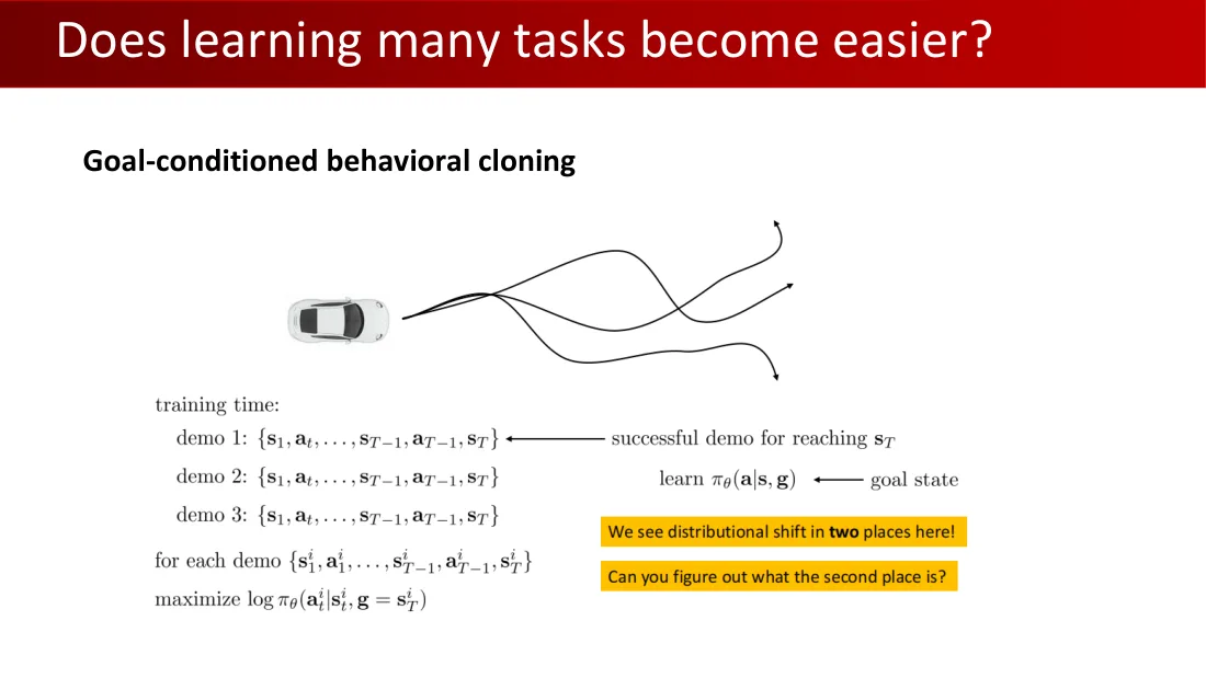
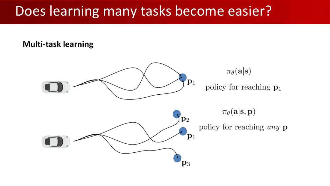
目标条件化行为克隆
训练时:
演示1:$\{s_1,a_1,\ldots,s_{T-1},a_{T-1},s_T^1\}$;演示2:$\{s_1,a_1,\ldots,s_{T-1},a_{T-1},s_T^2\}$;演示3:$\{s_1,a_1,\ldots,s_{T-1},a_{T-1},s_T^3\}$。
到达$s_T$的成功演示;学习$\pi_\theta(a\mid s,g)$;g为目标状态。
对每个演示$\{s_1^i,a_1^i,\ldots,s_{T-1}^i,a_{T-1}^i,s_T^i\}$,最大化$\log\pi_\theta(a_t^i\mid s_t^i,g=s_T^i)$。
这里有两处分布偏移!你能指出第二处吗?
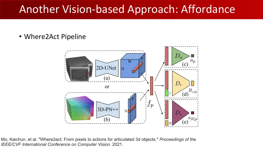
Where2Act管线。
Lecture 08 · PDF p72
Lecture 08 · PDF p73
Lecture 08 · PDF p74
Lecture 08 · PDF p75
Lecture 08 · PDF p76
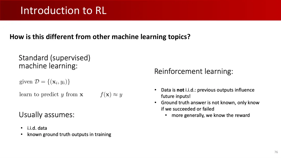
Lecture 08 · PDF p77
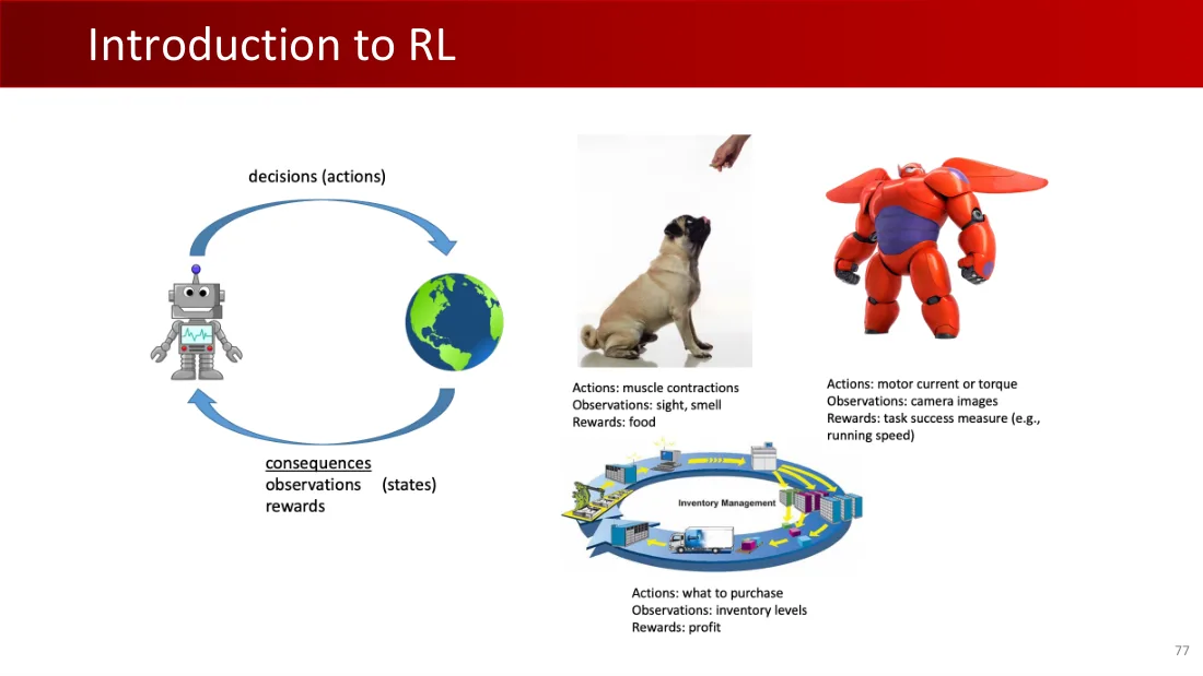
Lecture 08 · PDF p78
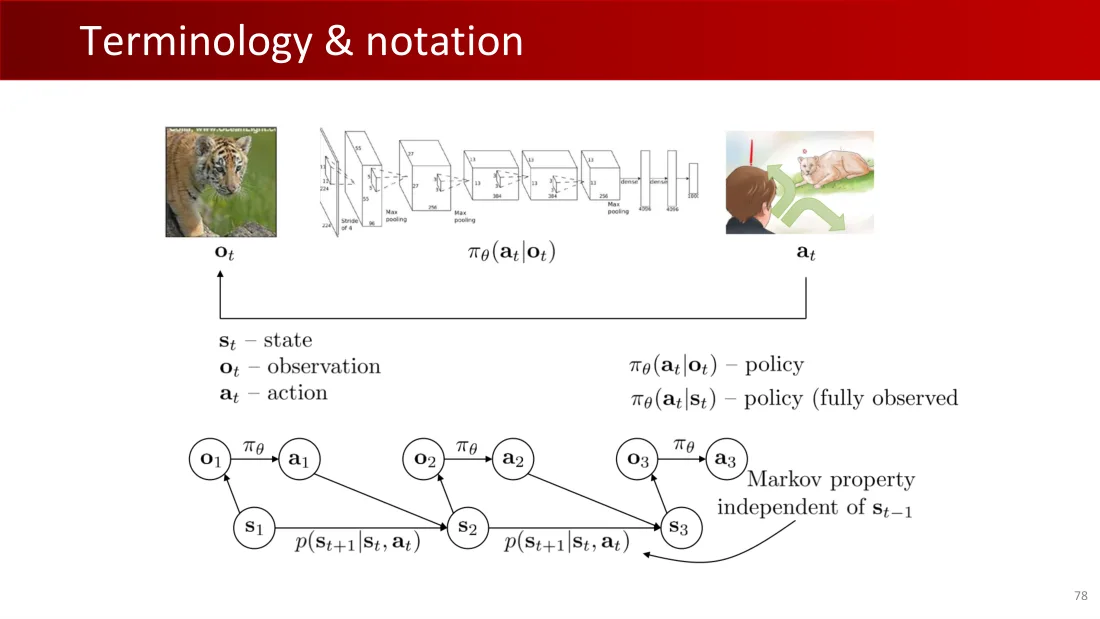
Lecture 08 · PDF p79
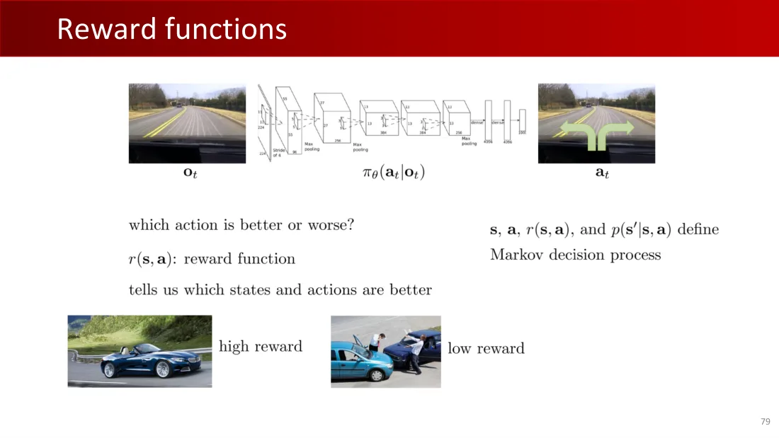
Lecture 08 · PDF p80
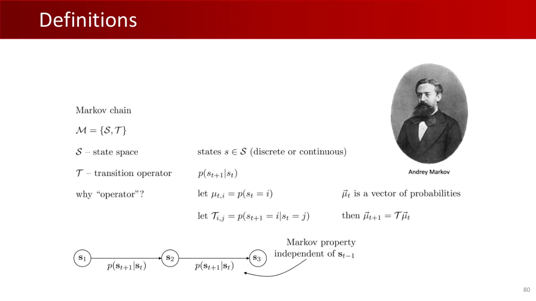
Lecture 08 · PDF p81
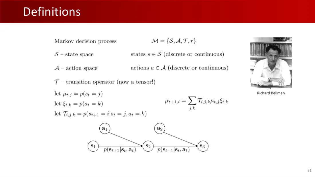
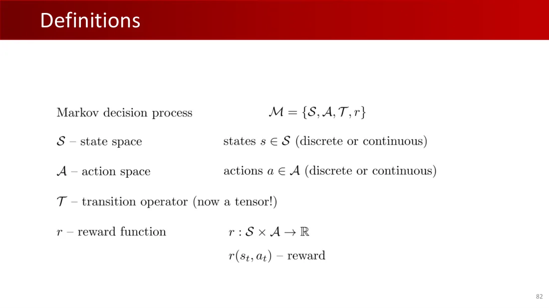
马尔可夫决策过程
$\mathcal M=\{S,A,\mathcal T,r\}$。
| 量 | 含义 |
|---|---|
| S:状态空间 | s∈S,离散或连续 |
| A:动作空间 | a∈A,离散或连续 |
| T:转移算子 | 现在是张量! |
令$\mu_{t,j}=p(s_t=j)$;令$\xi_{t,k}=p(a_t=k)$;令$\mathcal T_{i,j,k}=p(s_{t+1}=i\mid s_t=j,a_t=k)$;$\mu_{t+1,i}=\sum_{j,k}\mathcal T_{i,j,k}\mu_{t,j}\xi_{t,k}$。
$p(s_{t+1}\mid s_t,a_t)$;Richard Bellman(理查德·贝尔曼)。
状态s₁、s₂、s₃。
Lecture 08 · PDF p82
Lecture 08 · PDF p83
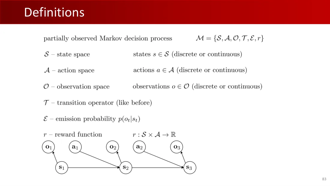
Lecture 08 · PDF p84
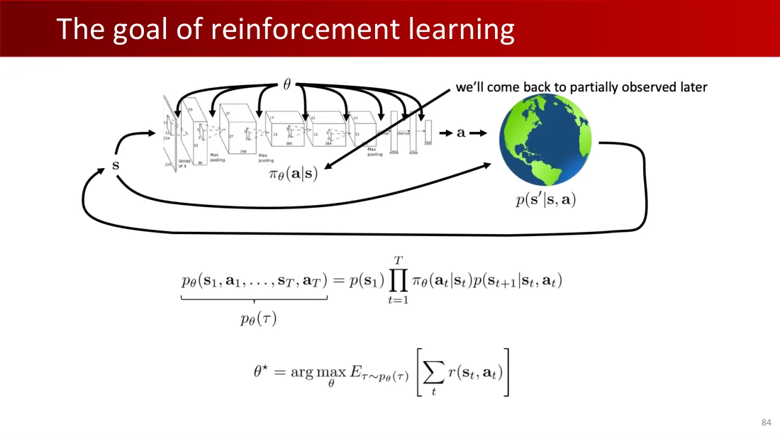
Lecture 08 · PDF p85
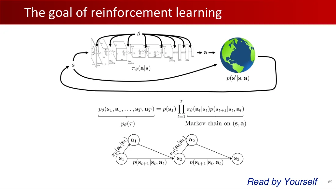
Lecture 08 · PDF p86
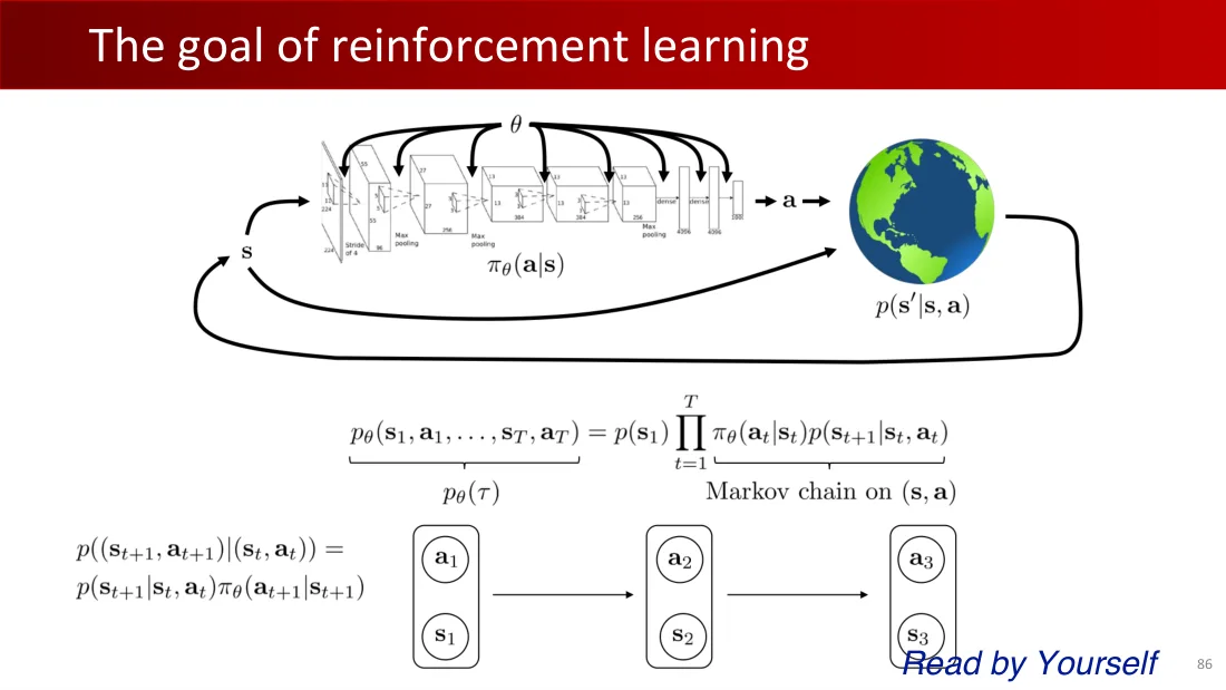
Lecture 08 · PDF p87
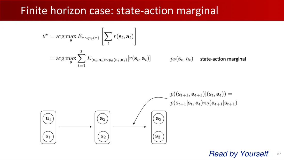
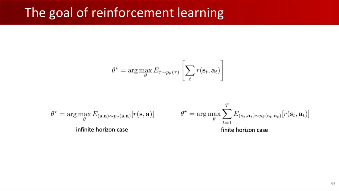
$\theta^*=\arg\max_\theta\mathbb E_{\tau\sim p_\theta(\tau)}[\sum_t r(s_t,a_t)]$。
$=\arg\max_\theta\sum_{t=1}^T\mathbb E_{(s_t,a_t)\sim p_\theta(s_t,a_t)}[r(s_t,a_t)]$。
$p_\theta(s_t,a_t)$:状态—动作边际分布。
$p((s_{t+1},a_{t+1})\mid(s_t,a_t))=p(s_{t+1}\mid s_t,a_t)\pi_\theta(a_{t+1}\mid s_{t+1})$。
自行阅读。
Lecture 08 · PDF p88

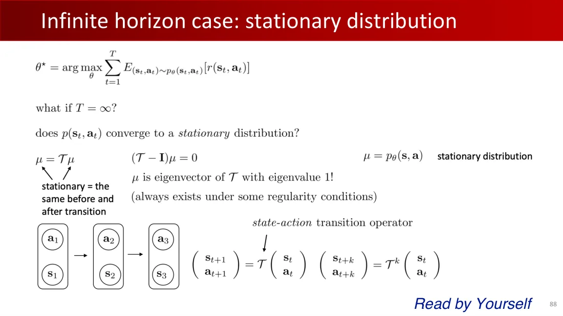
$\theta^*=\arg\max_\theta\sum_{t=1}^T\mathbb E_{(s_t,a_t)\sim p_\theta(s_t,a_t)}[r(s_t,a_t)]$。
如果T=∞呢?p(sₜ,aₜ)会收敛到平稳分布吗?
$\mu=\mathcal T\mu$;$(\mathcal T-I)\mu=0$;$\mu=p_\theta(s,a)$:平稳分布。
平稳=转移前后相同。μ是T的特征值1对应的特征向量!(在一定正则条件下总是存在。)
状态—动作转移算子:$\binom{s_{t+1}}{a_{t+1}}=\mathcal T\binom{s_t}{a_t}$;$\binom{s_{t+k}}{a_{t+k}}=\mathcal T^k\binom{s_t}{a_t}$。
自行阅读。
Lecture 08 · PDF p89

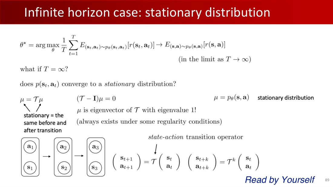
$\theta^*=\arg\max_\theta\frac1T\sum_{t=1}^T\mathbb E_{(s_t,a_t)\sim p_\theta(s_t,a_t)}[r(s_t,a_t)]\longrightarrow\mathbb E_{(s,a)\sim p_\theta(s,a)}[r(s,a)]$,当$T\to\infty$。
如果T=∞呢?p(sₜ,aₜ)会收敛到平稳分布吗?
$\mu=\mathcal T\mu$;$(\mathcal T-I)\mu=0$;$\mu=p_\theta(s,a)$:平稳分布。
平稳=转移前后相同。μ是T的特征值1对应的特征向量!(在一定正则条件下总是存在。)
状态—动作转移算子:$\binom{s_{t+1}}{a_{t+1}}=\mathcal T\binom{s_t}{a_t}$;$\binom{s_{t+k}}{a_{t+k}}=\mathcal T^k\binom{s_t}{a_t}$。
自行阅读。
Lecture 08 · PDF p90

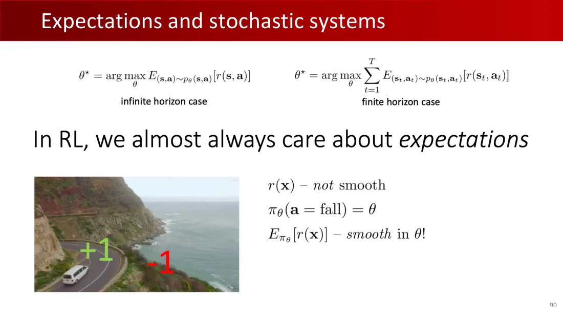
$\theta^*=\arg\max_\theta\mathbb E_{(s,a)\sim p_\theta(s,a)}[r(s,a)]$。无限时域情形。
$\theta^*=\arg\max_\theta\sum_{t=1}^T\mathbb E_{(s_t,a_t)\sim p_\theta(s_t,a_t)}[r(s_t,a_t)]$。有限时域情形。
强化学习中,我们几乎总是关心期望
$r(x)$:不平滑。$\pi_\theta(a=\text{坠落})=\theta$。$\mathbb E_{\pi_\theta}[r(x)]$:关于θ平滑!
奖励:+1、−1。
Lecture 08 · PDF p91
Lecture 08 · PDF p92
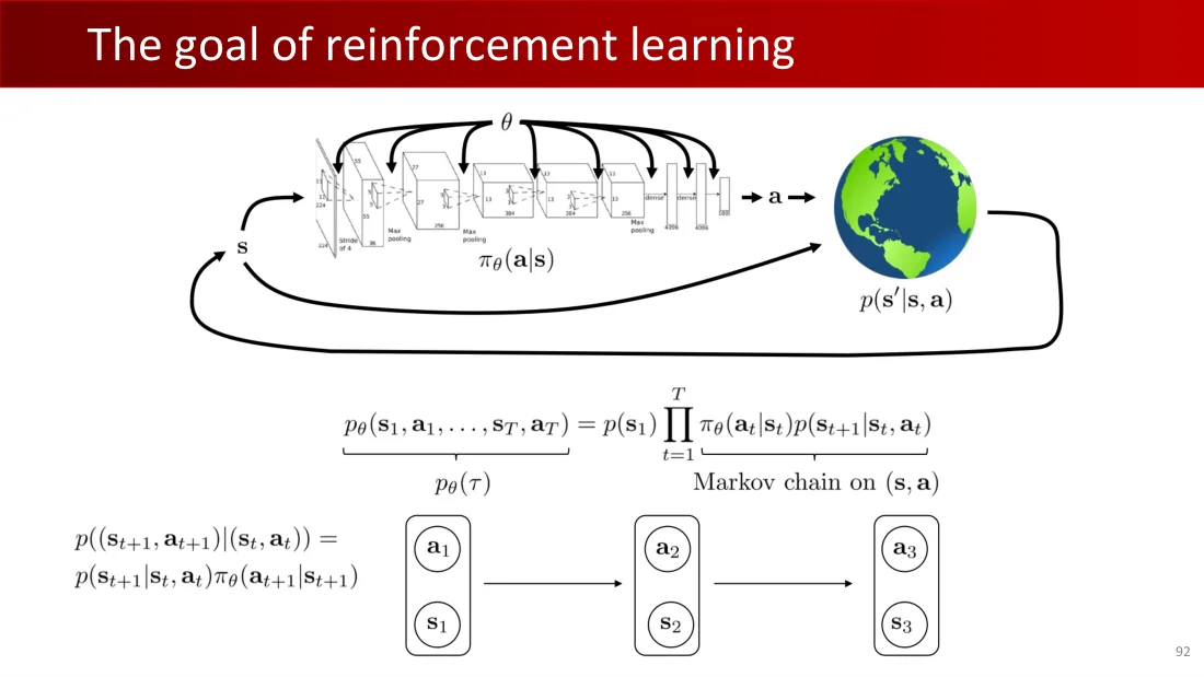
Lecture 08 · PDF p93
Lecture 08 · PDF p94
Lecture 08 · PDF p95
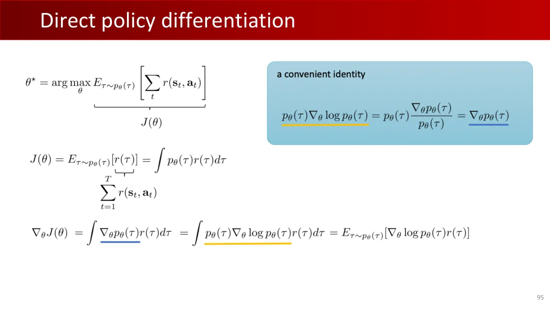
$\theta^*=\arg\max_\theta\mathbb E_{\tau\sim p_\theta(\tau)}[\sum_t r(s_t,a_t)]$。
J(θ)
$J(\theta)=\mathbb E_{\tau\sim p_\theta(\tau)}[r(\tau)]=\int p_\theta(\tau)r(\tau)d\tau$;$r(\tau)=\sum_{t=1}^Tr(s_t,a_t)$。
一个方便的恒等式
$p_\theta(\tau)\nabla_\theta\log p_\theta(\tau)=p_\theta(\tau)\frac{\nabla_\theta p_\theta(\tau)}{p_\theta(\tau)}=\nabla_\theta p_\theta(\tau)$。
$\nabla_\theta J(\theta)=\int\nabla_\theta p_\theta(\tau)r(\tau)d\tau=\int p_\theta(\tau)\nabla_\theta\log p_\theta(\tau)r(\tau)d\tau=\mathbb E_{\tau\sim p_\theta(\tau)}[\nabla_\theta\log p_\theta(\tau)r(\tau)]$。
Lecture 08 · PDF p96

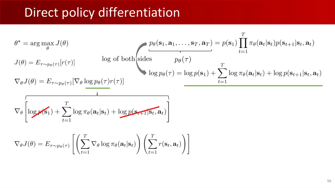
$\theta^*=\arg\max_\theta J(\theta)$;$J(\theta)=\mathbb E_{\tau\sim p_\theta(\tau)}[r(\tau)]$。
$\nabla_\theta J(\theta)=\mathbb E_{\tau\sim p_\theta(\tau)}[\nabla_\theta\log p_\theta(\tau)r(\tau)]$。
$p_\theta(s_1,a_1,\ldots,s_T,a_T)=p(s_1)\prod_{t=1}^T\pi_\theta(a_t\mid s_t)p(s_{t+1}\mid s_t,a_t)=p_\theta(\tau)$。
两边取对数:
$\log p_\theta(\tau)=\log p(s_1)+\sum_{t=1}^T[\log\pi_\theta(a_t\mid s_t)+\log p(s_{t+1}\mid s_t,a_t)]$。
$\nabla_\theta[\log p(s_1)+\sum_{t=1}^T\log\pi_\theta(a_t\mid s_t)+\log p(s_{t+1}\mid s_t,a_t)]$。
$\nabla_\theta J(\theta)=\mathbb E_{\tau\sim p_\theta(\tau)}[(\sum_{t=1}^T\nabla_\theta\log\pi_\theta(a_t\mid s_t))(\sum_{t=1}^T r(s_t,a_t))]$。
Lecture 08 · PDF p97

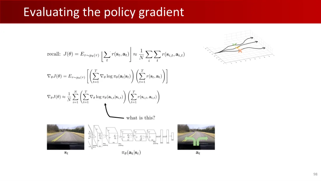
回顾:
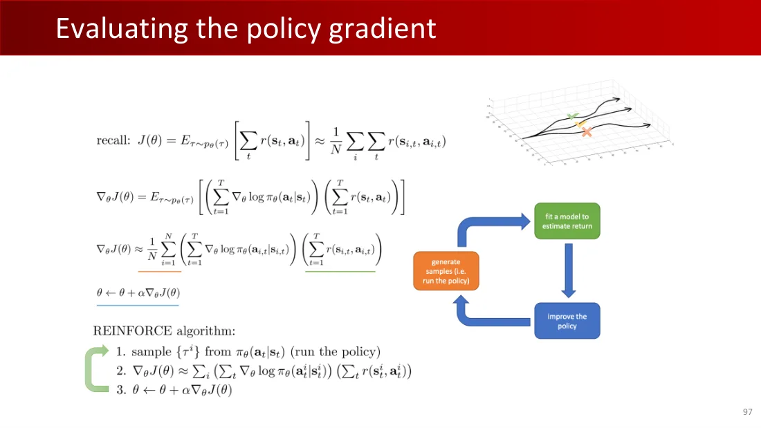
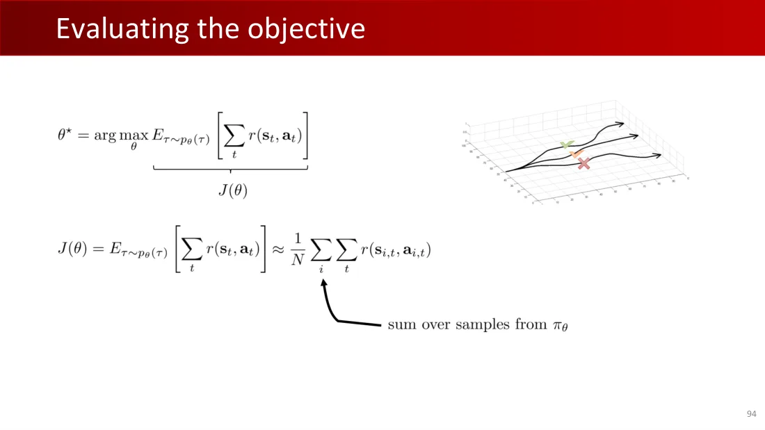
$J(\theta)=\mathbb E_{\tau\sim p_\theta(\tau)}[\sum_t r(s_t,a_t)]\approx\frac1N\sum_i\sum_t r(s_{i,t},a_{i,t})$。
$\nabla_\theta J(\theta)=\mathbb E_{\tau\sim p_\theta(\tau)}[(\sum_{t=1}^T\nabla_\theta\log\pi_\theta(a_t\mid s_t))(\sum_{t=1}^T r(s_t,a_t))]$。
$\nabla_\theta J(\theta)\approx\frac1N\sum_{i=1}^N(\sum_{t=1}^T\nabla_\theta\log\pi_\theta(a_{i,t}\mid s_{i,t}))(\sum_{t=1}^T r(s_{i,t},a_{i,t}))$。
$\theta\leftarrow\theta+\alpha\nabla_\theta J(\theta)$。
生成样本(即执行策略) → 拟合模型以估计回报 → 改进策略。
REINFORCE算法
- 从$\pi_\theta(a_t\mid s_t)$采样$\{\tau^i\}$(执行该策略)。
- $\nabla_\theta J(\theta)\approx\frac1N\sum_{i=1}^N(\sum_{t=1}^T\nabla_\theta\log\pi_\theta(a_{i,t}\mid s_{i,t}))(\sum_{t=1}^T r(s_{i,t},a_{i,t}))$。
- $\theta\leftarrow\theta+\alpha\nabla_\theta J(\theta)$。
Lecture 08 · PDF p98

回顾:
$J(\theta)=\mathbb E_{\tau\sim p_\theta(\tau)}[\sum_t r(s_t,a_t)]\approx\frac1N\sum_i\sum_t r(s_{i,t},a_{i,t})$。
$\nabla_\theta J(\theta)=\mathbb E_{\tau\sim p_\theta(\tau)}[(\sum_{t=1}^T\nabla_\theta\log\pi_\theta(a_t\mid s_t))(\sum_{t=1}^T r(s_t,a_t))]$。
$\nabla_\theta J(\theta)\approx\frac1N\sum_{i=1}^N(\sum_{t=1}^T\nabla_\theta\log\pi_\theta(a_{i,t}\mid s_{i,t}))(\sum_{t=1}^T r(s_{i,t},a_{i,t}))$。
这是什么?
sₜ → πθ(aₜ|sₜ) → aₜ。
Lecture 08 · PDF p99

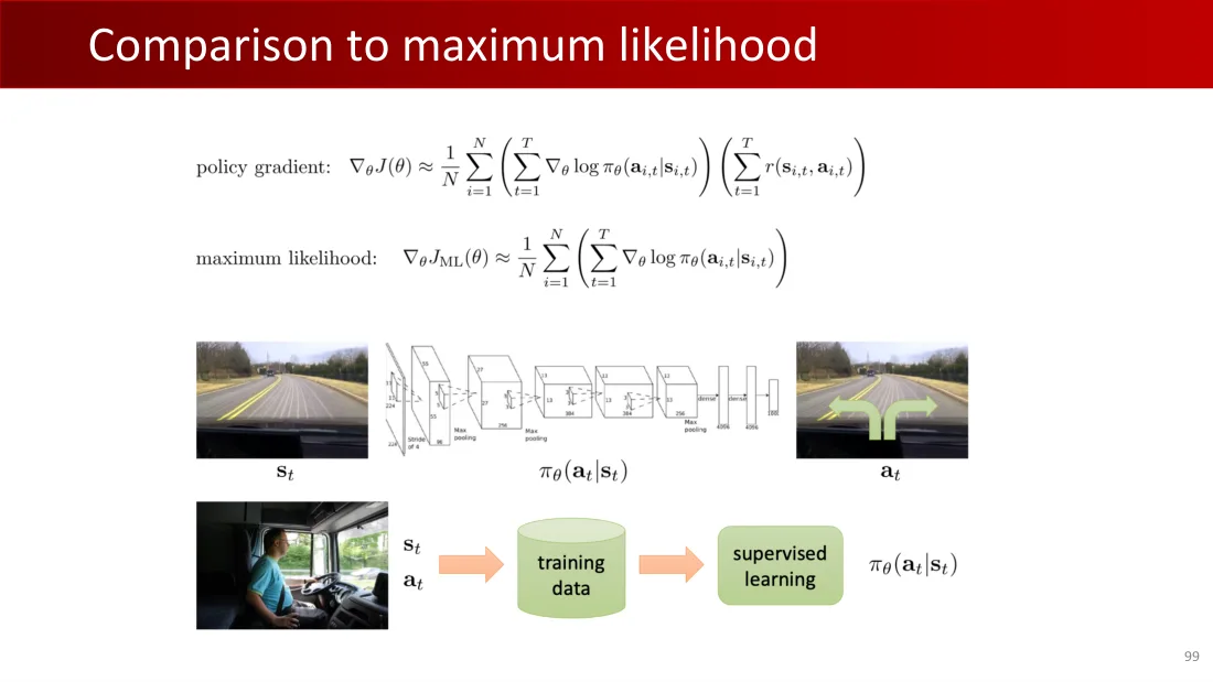
策略梯度:
$\nabla_\theta J(\theta)\approx\frac1N\sum_{i=1}^N(\sum_{t=1}^T\nabla_\theta\log\pi_\theta(a_{i,t}\mid s_{i,t}))(\sum_{t=1}^T r(s_{i,t},a_{i,t}))$。
最大似然:
$\nabla_\theta J_{ML}(\theta)\approx\frac1N\sum_{i=1}^N(\sum_{t=1}^T\nabla_\theta\log\pi_\theta(a_{i,t}\mid s_{i,t}))$。
sₜ、aₜ → 训练数据 → 监督学习 → πθ(aₜ|sₜ)。
Lecture 08 · PDF p100

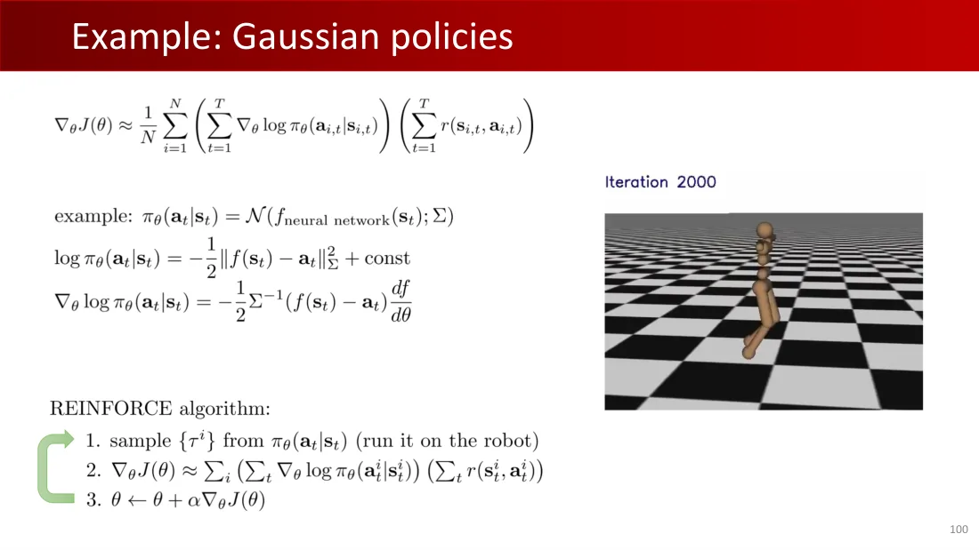
$\nabla_\theta J(\theta)\approx\frac1N\sum_{i=1}^N(\sum_{t=1}^T\nabla_\theta\log\pi_\theta(a_{i,t}\mid s_{i,t}))(\sum_{t=1}^T r(s_{i,t},a_{i,t}))$。
例:$\pi_\theta(a_t\mid s_t)=\mathcal N(f_{neural\ network}(s_t);\Sigma)$。
$\log\pi_\theta(a_t\mid s_t)=-\frac12\|f(s_t)-a_t\|_\Sigma^2+\text{常数}$。
$\nabla_\theta\log\pi_\theta(a_t\mid s_t)=-\frac12\Sigma^{-1}(f(s_t)-a_t)\frac{df}{d\theta}$。
第2000次迭代。
REINFORCE算法
- 从$\pi_\theta(a_t\mid s_t)$采样$\{\tau^i\}$(执行该策略)。
- $\nabla_\theta J(\theta)\approx\frac1N\sum_{i=1}^N(\sum_{t=1}^T\nabla_\theta\log\pi_\theta(a_{i,t}\mid s_{i,t}))(\sum_{t=1}^T r(s_{i,t},a_{i,t}))$。
- $\theta\leftarrow\theta+\alpha\nabla_\theta J(\theta)$。
Lecture 08 · PDF p101

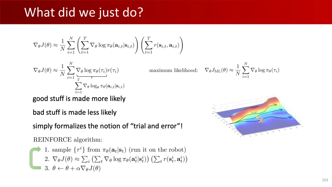
$\nabla_\theta J(\theta)\approx\frac1N\sum_{i=1}^N(\sum_{t=1}^T\nabla_\theta\log\pi_\theta(a_{i,t}\mid s_{i,t}))(\sum_{t=1}^T r(s_{i,t},a_{i,t}))$。
$\nabla_\theta J(\theta)\approx\frac1N\sum_{i=1}^N\nabla_\theta\log p_\theta(\tau)r(\tau)$。
$\nabla_\theta\log p_\theta(\tau)=\sum_{t=1}^T\nabla_\theta\log\pi_\theta(a_{i,t}\mid s_{i,t})$。
最大似然:$\nabla_\theta J_{ML}(\theta)\approx\frac1N\sum_{i=1}^N\nabla_\theta\log p_\theta(\tau)$。
让好行为更可能发生。让坏行为更不可能发生。
只是把“试错”的概念形式化!
REINFORCE算法
- 从$\pi_\theta(a_t\mid s_t)$采样$\{\tau^i\}$(执行该策略)。
- $\nabla_\theta J(\theta)\approx\frac1N\sum_{i=1}^N(\sum_{t=1}^T\nabla_\theta\log\pi_\theta(a_{i,t}\mid s_{i,t}))(\sum_{t=1}^T r(s_{i,t},a_{i,t}))$。
- $\theta\leftarrow\theta+\alpha\nabla_\theta J(\theta)$。
Lecture 08 · PDF p102
Lecture 08 · PDF p103
Lecture 08 · PDF p104
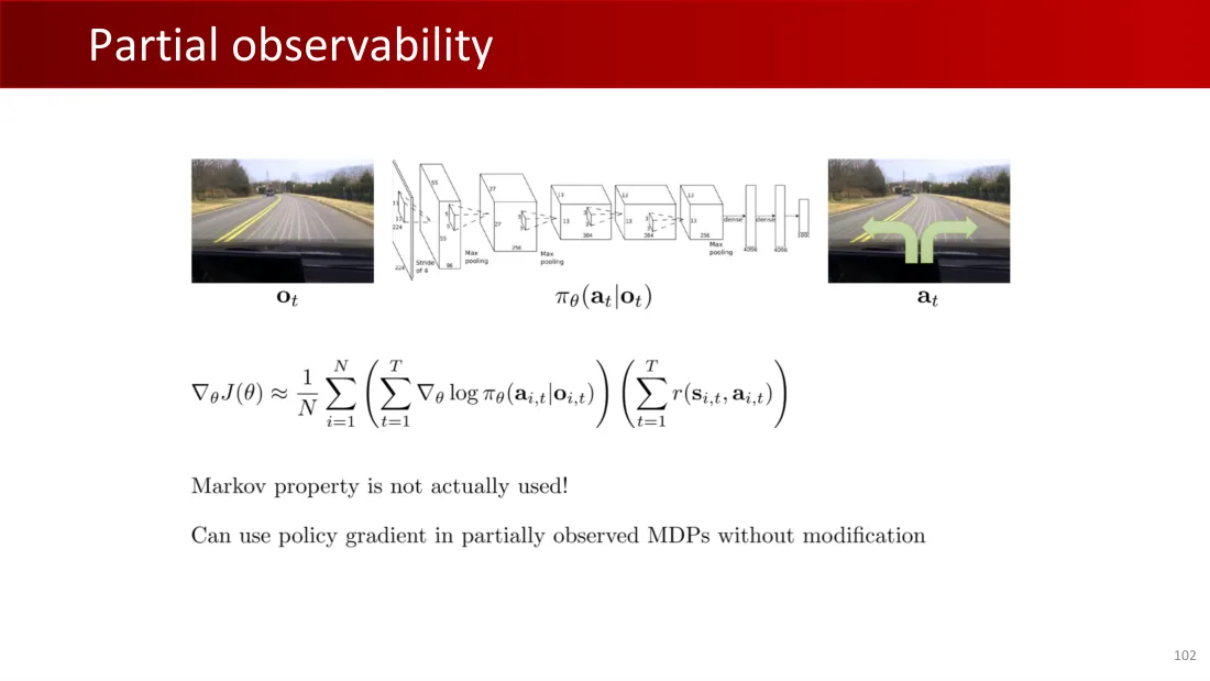
Lecture 08 · PDF p105