第5章 · 原课件与完整中文翻译
上方为英文原页,下方为对应的完整中文翻译,标题、正文、图内文字和公式按原页顺序排列。
页号按PDF顺序。原课件的历史日期、学期、课堂安排和研究结论按原文保留;相关概念与适用条件见教程正文。符号、代码、作者姓名及便于检索的专有名称保留原文。
Lecture 05 · 71页
Lecture 05 · PDF p1
Lecture 05 · PDF p2
Lecture 05 · PDF p3
Lecture 05 · PDF p4
Lecture 05 · PDF p5
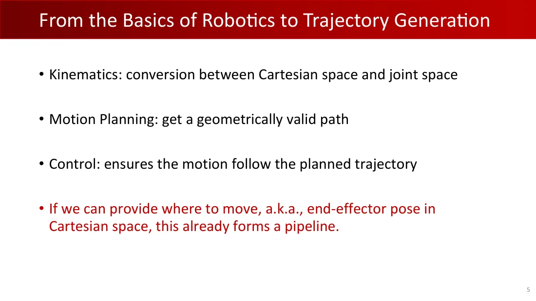
Lecture 05 · PDF p6
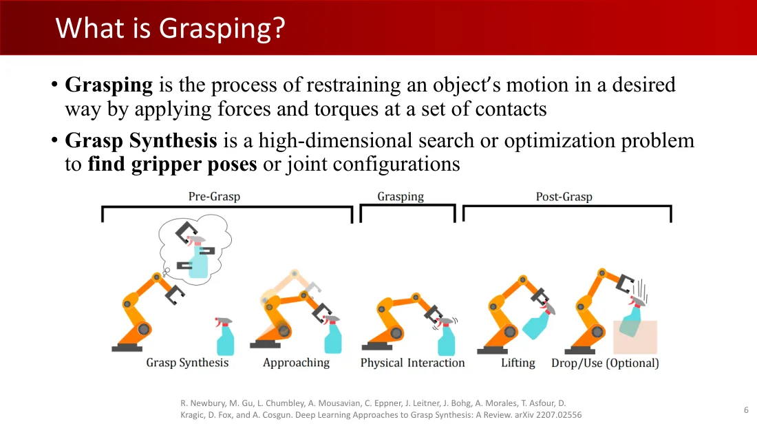
Lecture 05 · PDF p7
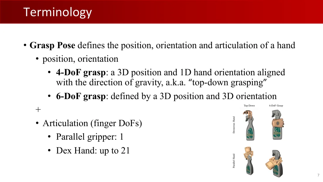
Lecture 05 · PDF p8
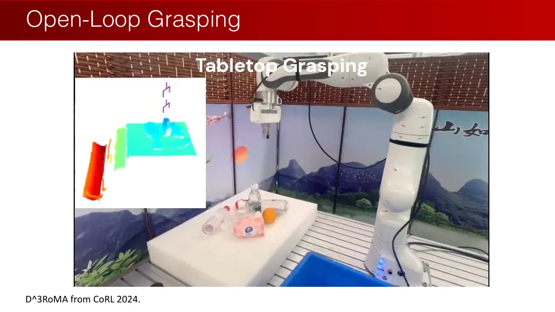
Lecture 05 · PDF p9
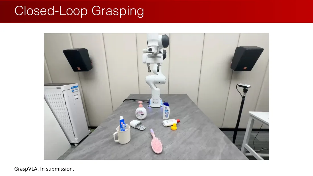
Lecture 05 · PDF p10
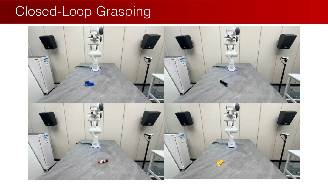
Lecture 05 · PDF p11
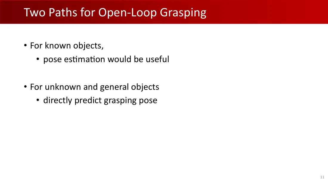
Lecture 05 · PDF p12
Lecture 05 · PDF p13
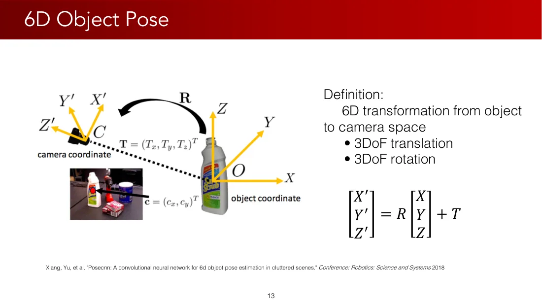
Lecture 05 · PDF p14
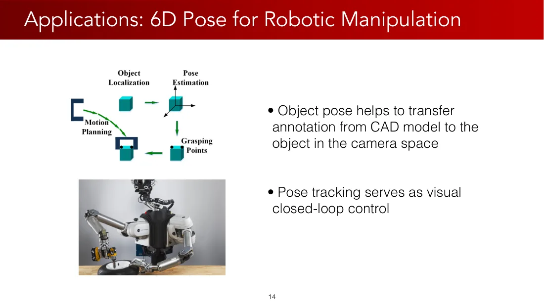
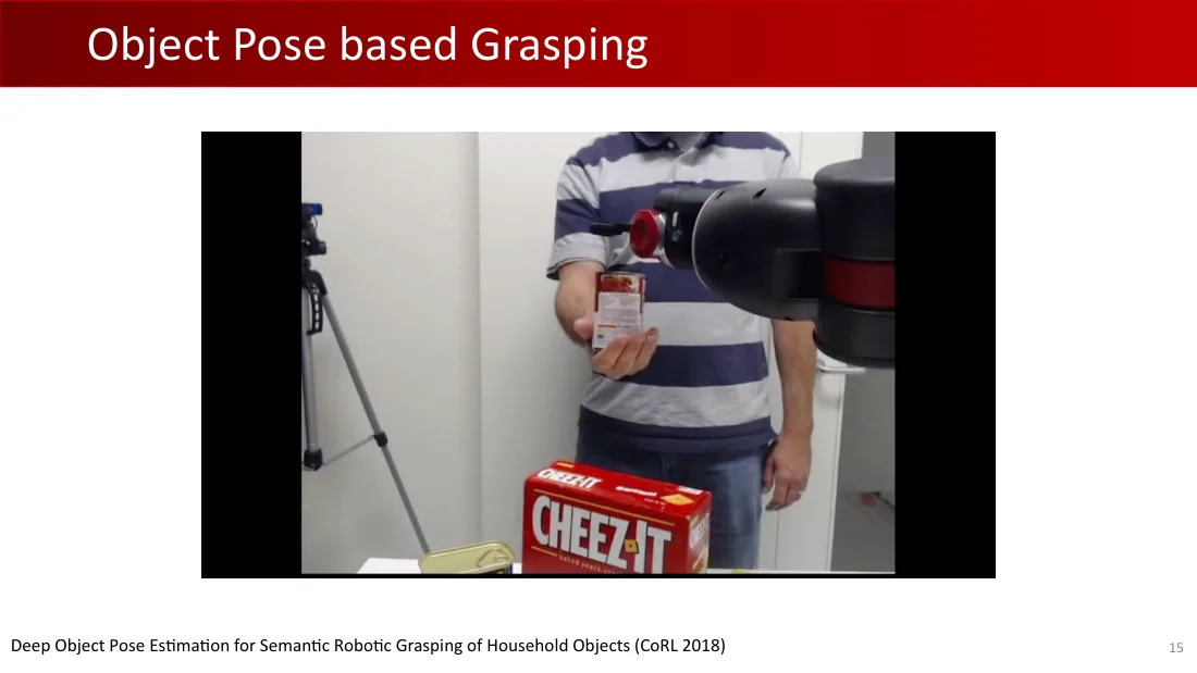
Lecture 05 · PDF p15
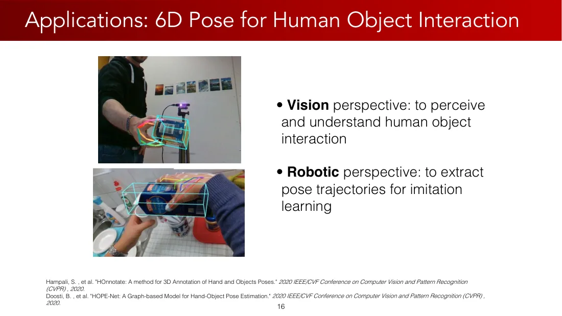
Lecture 05 · PDF p16
Lecture 05 · PDF p17
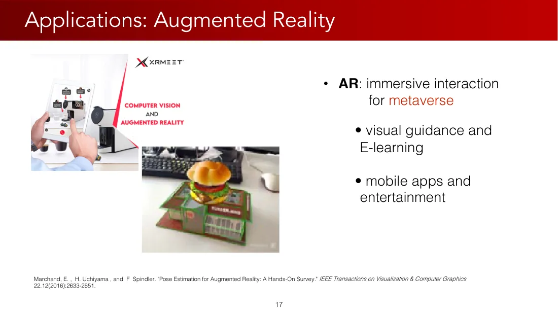
Lecture 05 · PDF p18
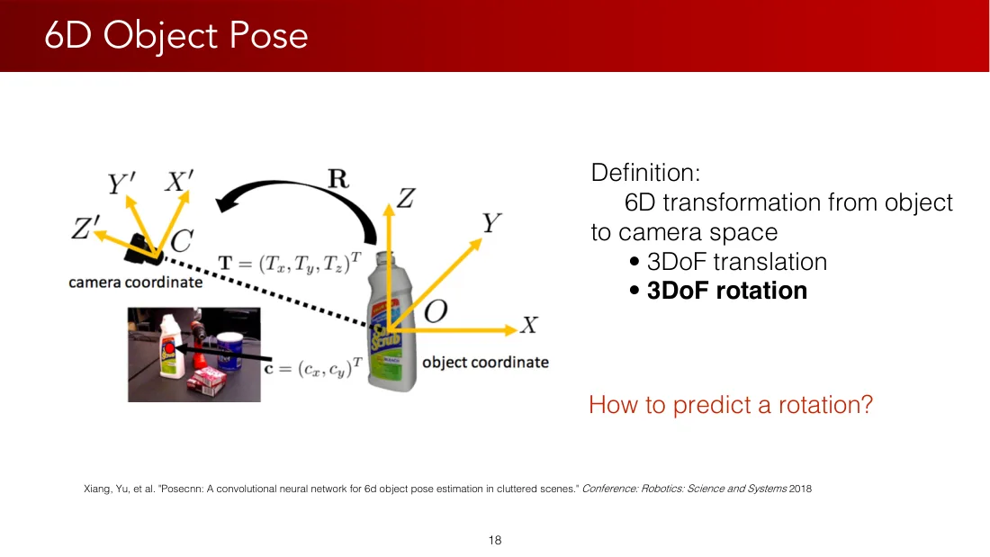
Lecture 05 · PDF p19
Lecture 05 · PDF p20
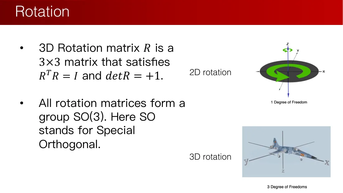
Lecture 05 · PDF p21
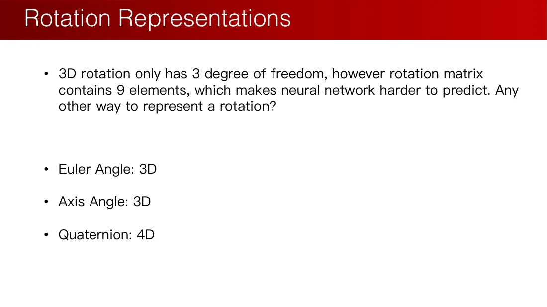
Lecture 05 · PDF p22
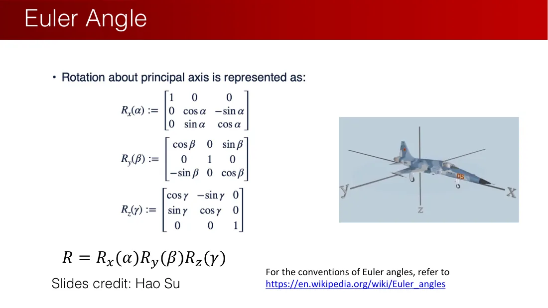
- 绕三个主坐标轴进行旋转。
\[R_x(\alpha)=\begin{bmatrix}1&0&0\\0&\cos\alpha&-\sin\alpha\\0&\sin\alpha&\cos\alpha\end{bmatrix}\]
\[R_y(\beta)=\begin{bmatrix}\cos\beta&0&\sin\beta\\0&1&0\\-\sin\beta&0&\cos\beta\end{bmatrix}\]
\[R_z(\gamma)=\begin{bmatrix}\cos\gamma&-\sin\gamma&0\\\sin\gamma&\cos\gamma&0\\0&0&1\end{bmatrix}\]
\[R=R_x(\alpha)R_y(\beta)R_z(\gamma)\]
幻灯片来源:Hao Su。欧拉角约定:https://en.wikipedia.org/wiki/Euler_angles。
Lecture 05 · PDF p23
Lecture 05 · PDF p24
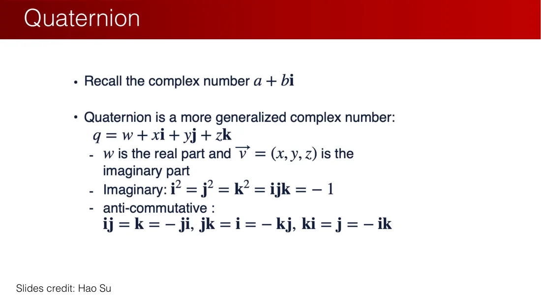
Lecture 05 · PDF p25
Lecture 05 · PDF p26
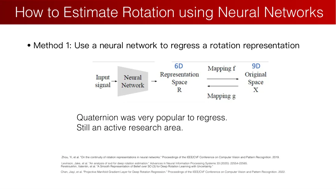
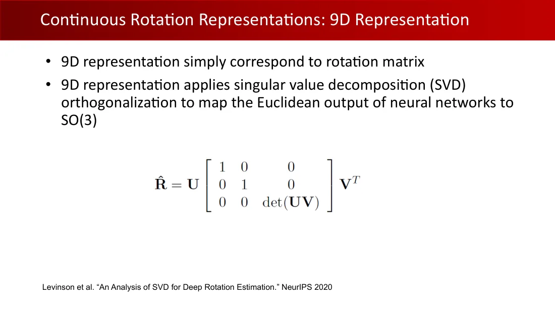
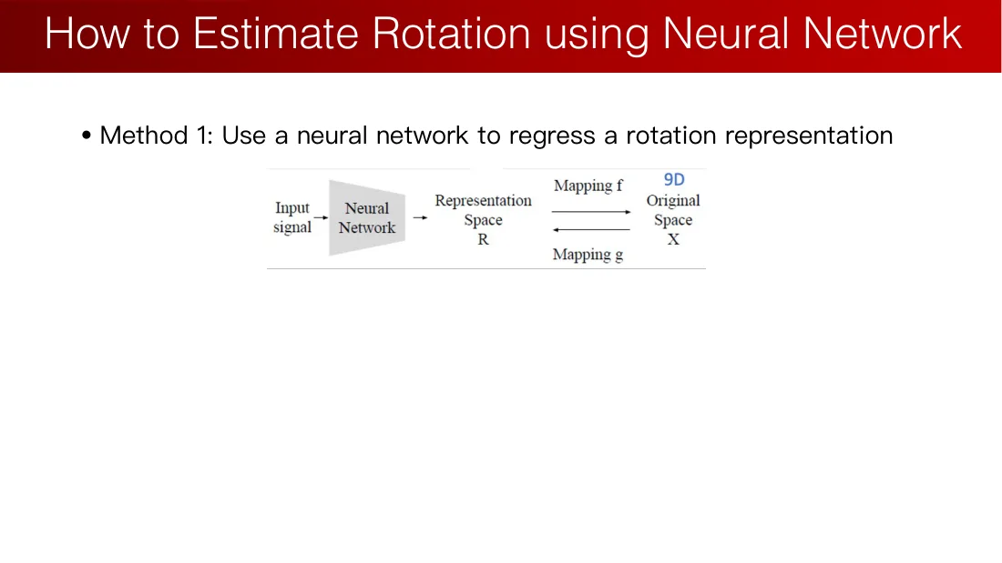
- 方法 1:使用神经网络回归一种旋转表示。
输入信号 → 神经网络 → 表示空间 R(6 维)→ 映射 f → 原空间 X(9 维);反向映射 g。
四元数曾是很流行的回归表示。该方向仍是活跃的研究领域。
Yi Zhou 等,《神经网络中旋转表示的连续性》,IEEE/CVF 计算机视觉与模式识别会议论文集,2019。
Jake Levinson 等,《深度旋转估计中 SVD 的分析》,Advances in Neural Information Processing Systems 33,2020,22554–22565。
Valentin Peretroukhin 等,《面向含不确定性的深度旋转学习的 SO(3) 上信念的平滑表示》。
Jiayi Chen 等,《用于深度旋转回归的投影流形梯度层》,IEEE/CVF 计算机视觉与模式识别会议论文集,2022。
Lecture 05 · PDF p27
Lecture 05 · PDF p28
Lecture 05 · PDF p29
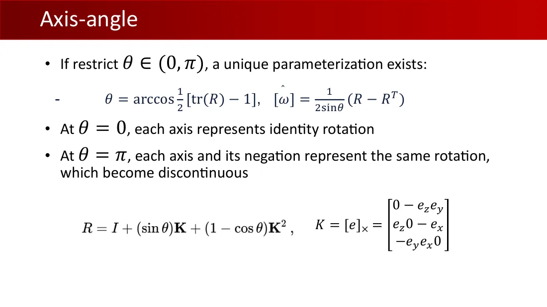
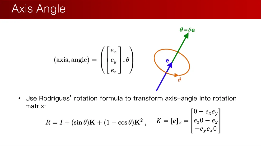
- 当 \(\theta\in(0,\pi)\) 时,表示唯一。
\[\theta=\arccos\left(\frac{\operatorname{tr}(R)-1}{2}\right)\]
\[[\omega]=\frac{R-R^{\mathsf T}}{2\sin\theta}\]
\(R=I+(\sin\theta)K+(1-\cos\theta)K^2\);\[K=[e]_\times=\begin{bmatrix}0&-e_z&e_y\\e_z&0&-e_x\\-e_y&e_x&0\end{bmatrix}\]
- \(\theta=0\) 时,任意旋转轴均对应单位旋转。
- \(\theta=\pi\) 时,旋转轴与其相反方向表示同一旋转,导致不连续。
Lecture 05 · PDF p30
Lecture 05 · PDF p31
Lecture 05 · PDF p32
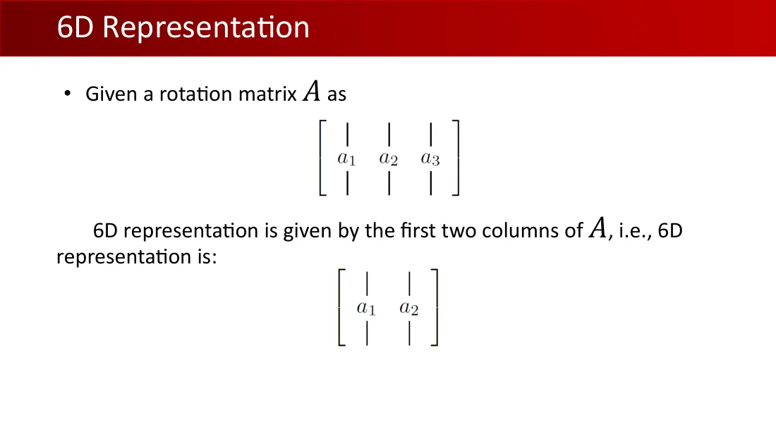
Lecture 05 · PDF p33
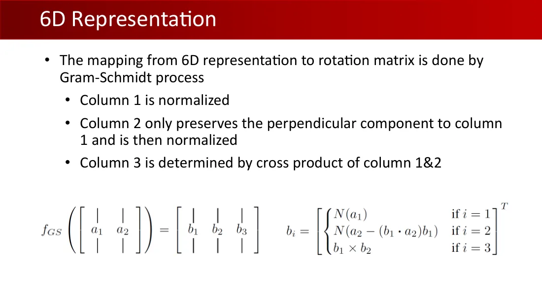
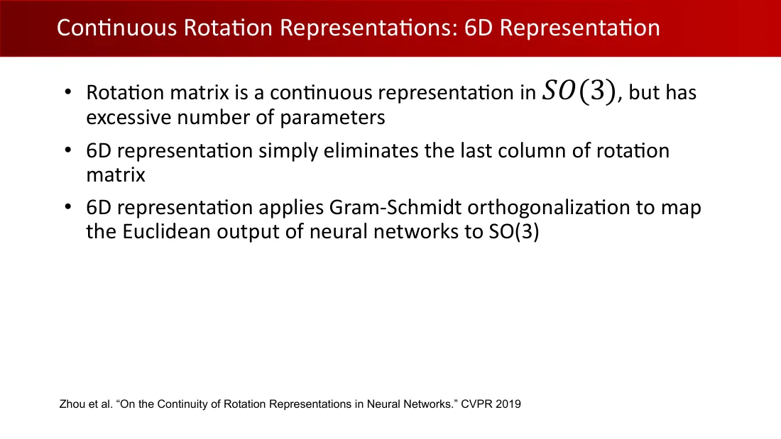
- 从 6 维表示到旋转矩阵的映射通过 Gram–Schmidt 过程完成。
- 将第 1 列归一化。
- 第 2 列只保留垂直于第 1 列的分量,然后归一化。
- 第 3 列由第 1、2 列的叉积确定。
\[f_{\mathrm{GS}}\!\left(\begin{bmatrix}a_1&a_2\end{bmatrix}\right)=\begin{bmatrix}b_1&b_2&b_3\end{bmatrix}\]
\[\begin{aligned}b_1&=N(a_1)\\b_2&=N\!\left(a_2-(b_1\cdot a_2)b_1\right)\\b_3&=b_1\times b_2\end{aligned}\]
Lecture 05 · PDF p34
Lecture 05 · PDF p35
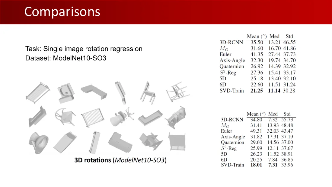
任务:单幅图像的旋转回归。数据集:ModelNet10-SO(3)。
| 方法 | 平均误差(°) | 中位误差(°) | 标准差(°) |
|---|---|---|---|
| 3D-RCNN | 35.50 | 13.21 | 46.55 |
| M_G | 31.60 | 16.70 | 41.86 |
| 欧拉角 | 41.35 | 27.44 | 37.73 |
| 轴角 | 32.30 | 19.74 | 34.70 |
| 四元数 | 26.92 | 14.39 | 32.92 |
| S²-Reg | 27.36 | 15.41 | 33.17 |
| 5D | 25.18 | 13.40 | 32.10 |
| 6D | 22.60 | 11.51 | 31.24 |
| SVD-Train | 21.25 | 11.14 | 30.28 |
| 方法 | 平均误差(°) | 中位误差(°) | 标准差(°) |
|---|---|---|---|
| 3D-RCNN | 34.80 | 7.32 | 55.73 |
| M_G | 31.41 | 13.93 | 48.48 |
| 欧拉角 | 49.31 | 32.03 | 43.47 |
| 轴角 | 31.82 | 17.31 | 37.19 |
| 四元数 | 29.60 | 14.56 | 37.00 |
| S²-Reg | 25.99 | 12.11 | 37.67 |
| 5D | 26.23 | 11.52 | 38.91 |
| 6D | 20.25 | 7.84 | 36.85 |
| SVD-Train | 18.01 | 7.31 | 33.96 |
来源:Jake Levinson 等,《旋转估计中 SVD 的分析》,NeurIPS 2020。
Lecture 05 · PDF p36
Lecture 05 · PDF p37
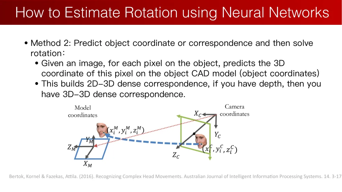
- 方法 2:预测物体坐标或点对应关系,再求解旋转。
- 给定图像,为物体上的每个像素预测它在物体 CAD 模型上的三维坐标,即物体坐标。
- 这样建立了稠密的 2D–3D 对应关系。如果有深度,就可以得到稠密的 3D–3D 对应关系。
模型坐标系;相机坐标系;\(x_m\)、\(y_m\)、\(z_m\);\(x_c\)、\(y_c\)、\(z_c\)。
Kornel Bertok、Attila Fazekas,《识别复杂的头部运动》,Australian Journal of Intelligent Information Processing Systems 14,2016,3–17。
Lecture 05 · PDF p38

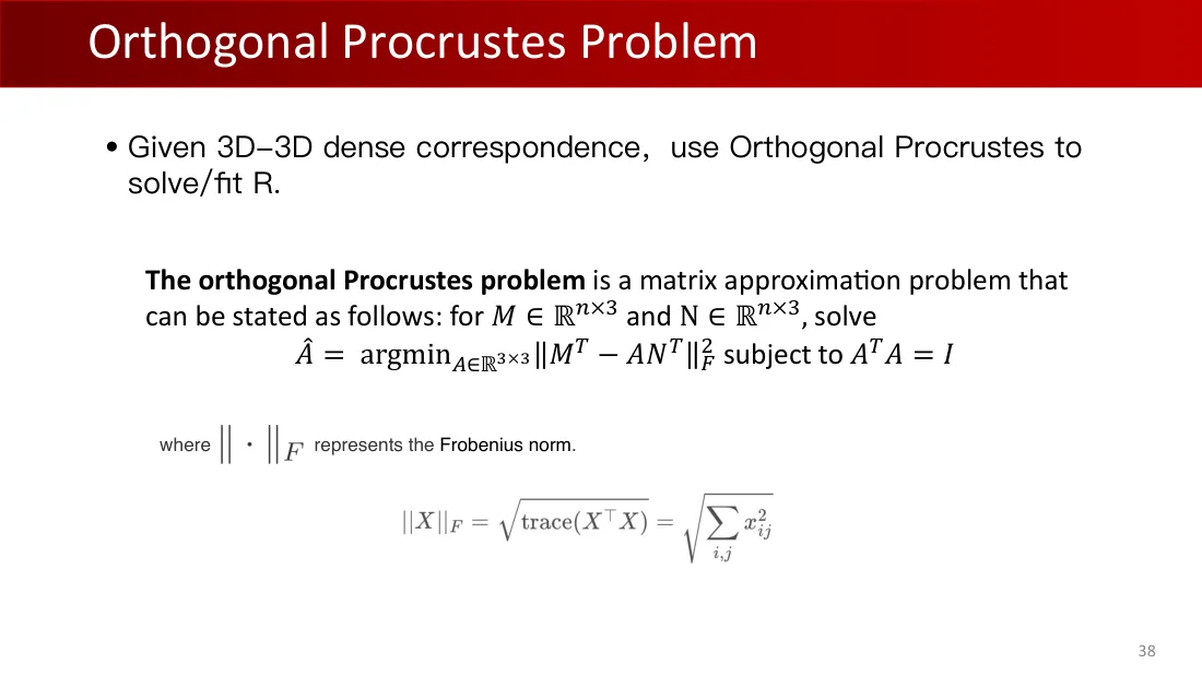
- 给定稠密的 3D–3D 对应关系,利用正交 Procrustes 问题求解/拟合 R。
正交 Procrustes 问题是一个矩阵近似问题,可表述为:对于 \(M,N\in\mathbb R^{n\times3}\),求解
\(\hat A=\operatorname*{argmin}_{A\in\mathbb R^{3\times3}}\left\|M^{\mathsf T}-AN^{\mathsf T}\right\|_F^2\),约束为 \(A^{\mathsf T}A=I\)。
其中 \(\|\cdot\|_F\) 表示 Frobenius 范数:\(\|X\|_F=\sqrt{\operatorname{tr}(X^{\mathsf T}X)}=\sqrt{\sum_{i,j}x_{ij}^2}\)。
Lecture 05 · PDF p39
Lecture 05 · PDF p40
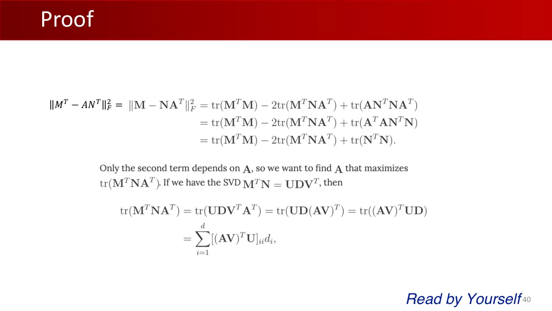
请自行阅读。
\[\|M^{\mathsf T}-AN^{\mathsf T}\|_F^2=\|M-NA^{\mathsf T}\|_F^2\]
\[=\operatorname{tr}(M^{\mathsf T}M)-2\operatorname{tr}(M^{\mathsf T}NA^{\mathsf T})+\operatorname{tr}(AN^{\mathsf T}NA^{\mathsf T})\]
\[=\operatorname{tr}(M^{\mathsf T}M)-2\operatorname{tr}(M^{\mathsf T}NA^{\mathsf T})+\operatorname{tr}(A^{\mathsf T}AN^{\mathsf T}N)\]
\[=\operatorname{tr}(M^{\mathsf T}M)-2\operatorname{tr}(M^{\mathsf T}NA^{\mathsf T})+\operatorname{tr}(N^{\mathsf T}N)\]
只有第二项依赖于 A,因此需要最大化 \(\operatorname{tr}(M^{\mathsf T}NA^{\mathsf T})\)。
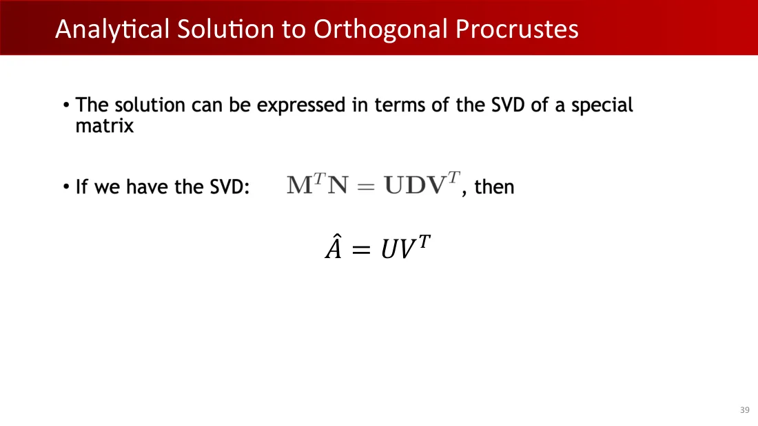
对 \(M^{\mathsf T}N=UDV^{\mathsf T}\) 进行 SVD:
\[\begin{aligned}\operatorname{tr}(M^{\mathsf T}NA^{\mathsf T})&=\operatorname{tr}(UDV^{\mathsf T}A^{\mathsf T})\\&=\operatorname{tr}(UD(AV)^{\mathsf T})\\&=\operatorname{tr}((AV)^{\mathsf T}UD)\\&=\sum_{i=1}^d[(AV)^{\mathsf T}U]_{ii}d_i\end{aligned}\]
Lecture 05 · PDF p41

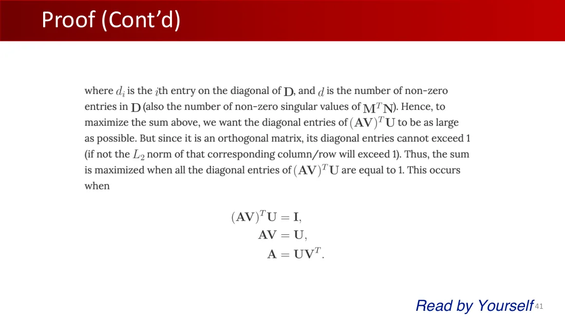
请自行阅读。
\(\sum_{i=1}^d[(AV)^{\mathsf T}U]_{ii}d_i\) 中,\(d_i\) 是 D 的第 i 个对角元素,d 为非零奇异值的数量;它们也是 \(M^{\mathsf T}N\) 的奇异值。
为了使这一和式最大,应让 \((AV)^{\mathsf T}U\) 的对角元素尽可能大。
正交矩阵的元素不能大于 1,否则某行或某列的 \(L_2\) 范数会大于 1。
所有对角元素都为 1 时,和式达到最大值。这发生在 \((AV)^{\mathsf T}U=I\) 时。
\(AV=U\),因此 \(A=UV^{\mathsf T}\)。
Lecture 05 · PDF p42
Lecture 05 · PDF p43
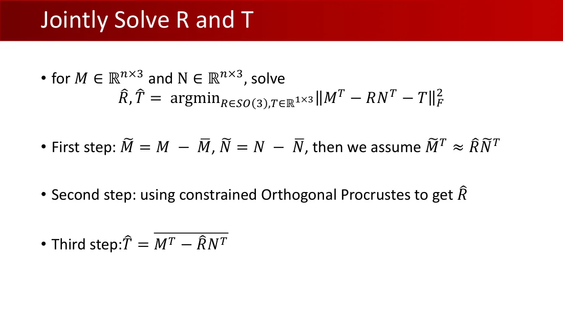
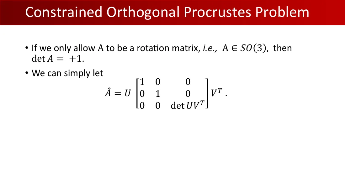
- 对于 \(M,N\in\mathbb R^{n\times3}\),求解:\(\hat R,\hat T=\operatorname*{argmin}_{\substack{R\in\mathrm{SO}(3)\\T\in\mathbb R^{1\times3}}}\left\|M^{\mathsf T}-RN^{\mathsf T}-T\right\|_F^2\)。
- 第一步:\(\tilde M=M-\bar M\),\(\tilde N=N-\bar N\);然后假设 \(\tilde M^{\mathsf T}\approx\hat R\tilde N^{\mathsf T}\)。
- 第二步:利用带约束的正交 Procrustes 问题得到 \(\hat R\)。
- 第三步:\(\hat T=\bar M^{\mathsf T}-\hat R\bar N^{\mathsf T}\)。
Lecture 05 · PDF p44
Lecture 05 · PDF p45
Lecture 05 · PDF p46
Lecture 05 · PDF p47
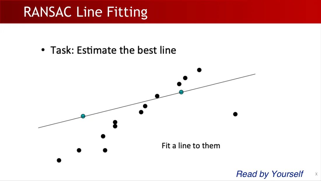
Lecture 05 · PDF p48
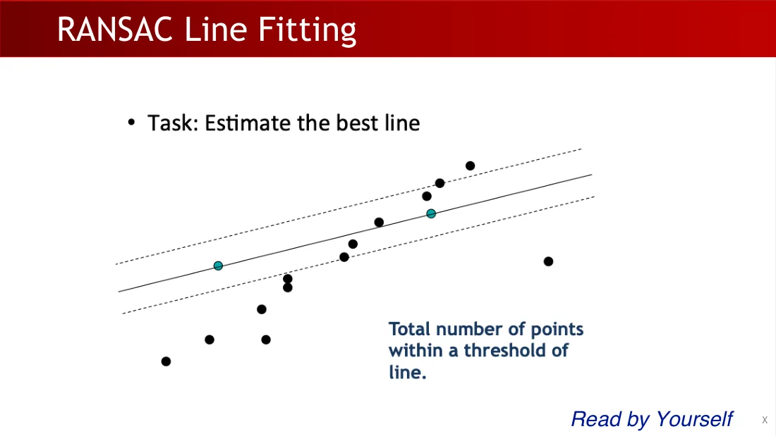
Lecture 05 · PDF p49
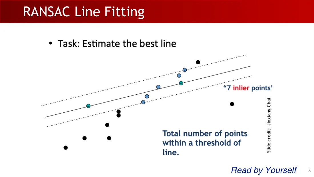
Lecture 05 · PDF p50
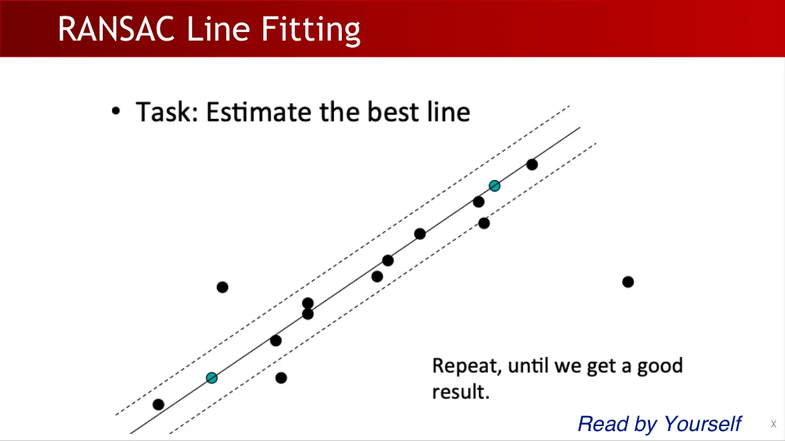
Lecture 05 · PDF p51
Lecture 05 · PDF p52
Lecture 05 · PDF p53
请自行阅读。
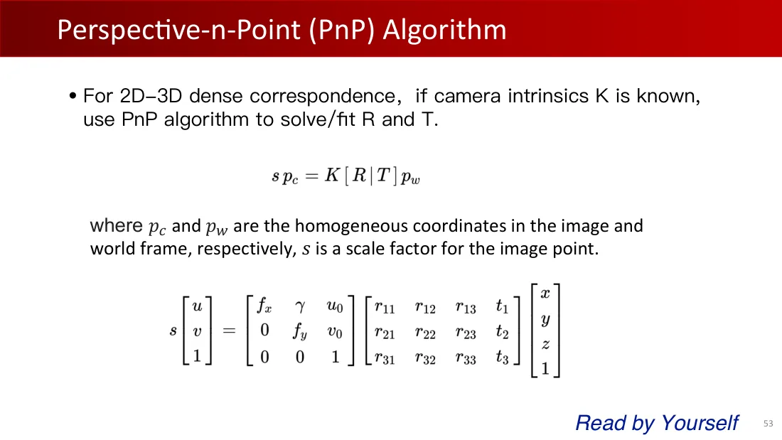
已知相机内参 K,通过 2D–3D 点对应求解 R 和 T。
\[sp_c=K\left[R\mid T\right]p_w\]
\(p_c\) 和 \(p_w\) 分别为图像坐标和世界坐标的齐次表示;s 为尺度因子。
\[s\begin{bmatrix}u\\v\\1\end{bmatrix}=\begin{bmatrix}f_x&\gamma&u_0\\0&f_y&v_0\\0&0&1\end{bmatrix}\times\begin{bmatrix}r_{11}&r_{12}&r_{13}&t_1\\r_{21}&r_{22}&r_{23}&t_2\\r_{31}&r_{32}&r_{33}&t_3\end{bmatrix}\times\begin{bmatrix}x\\y\\z\\1\end{bmatrix}\]
Lecture 05 · PDF p54
Lecture 05 · PDF p55
Lecture 05 · PDF p56
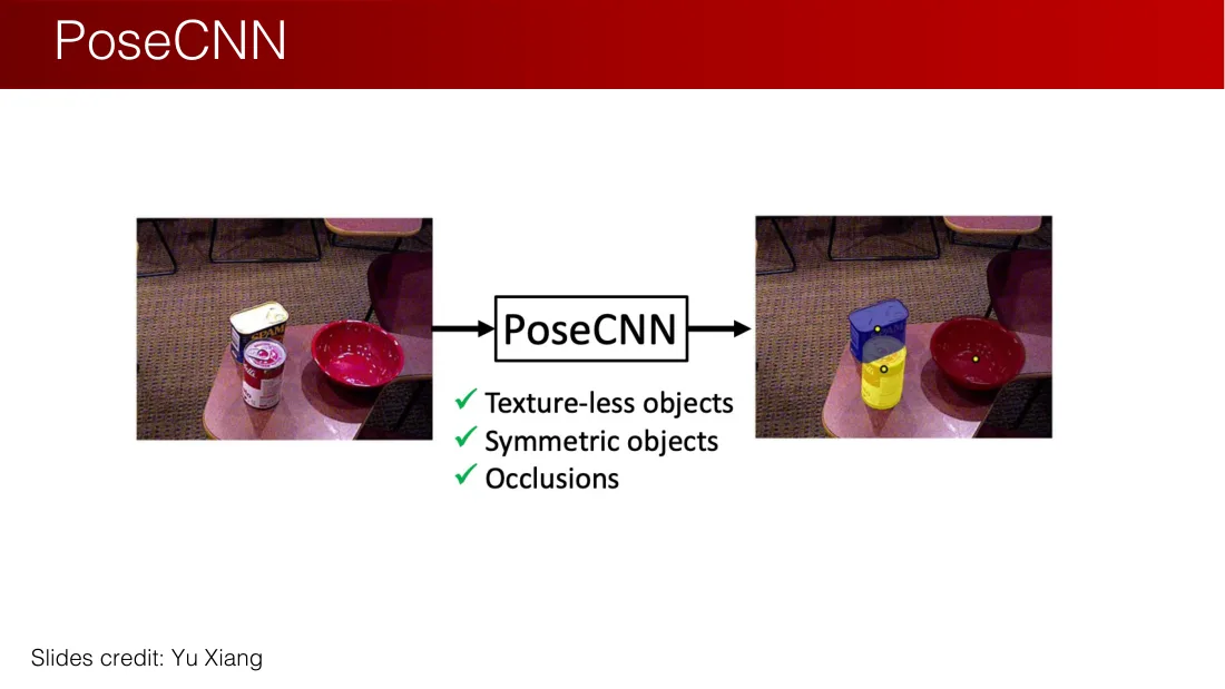
Lecture 05 · PDF p57
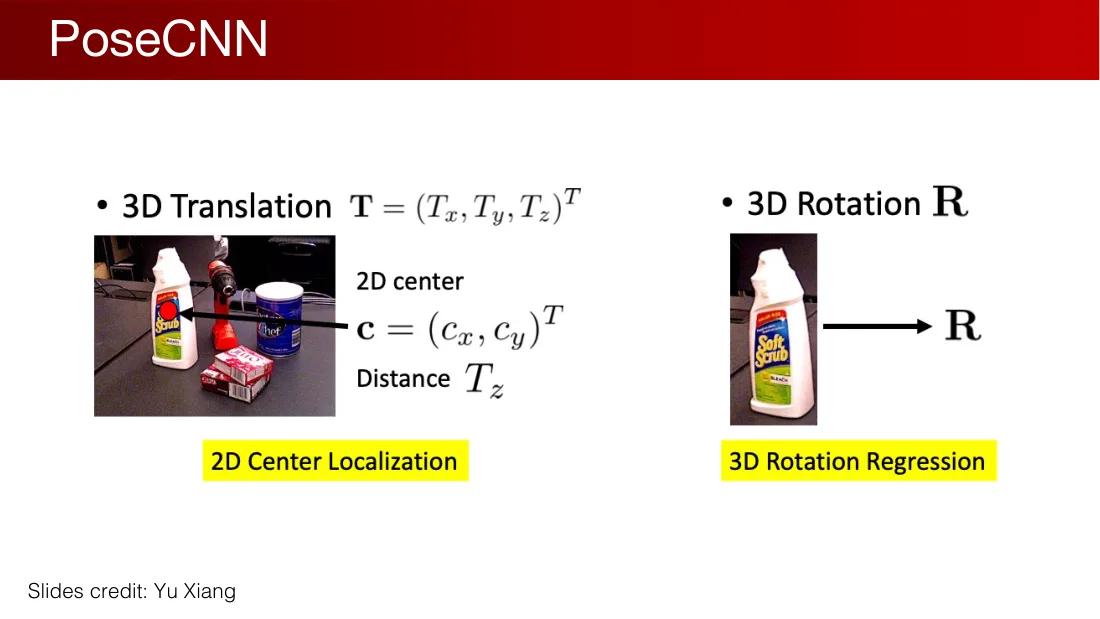
Lecture 05 · PDF p58
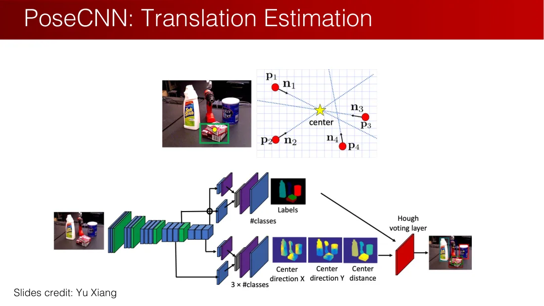
Lecture 05 · PDF p59
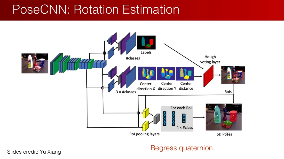
Lecture 05 · PDF p60
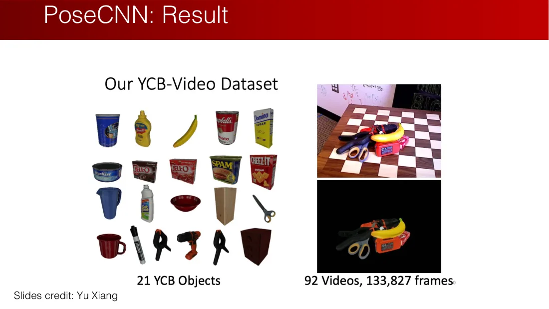
Lecture 05 · PDF p61
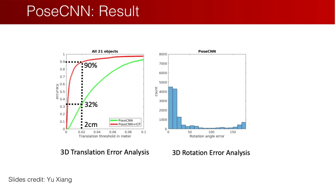
Lecture 05 · PDF p62
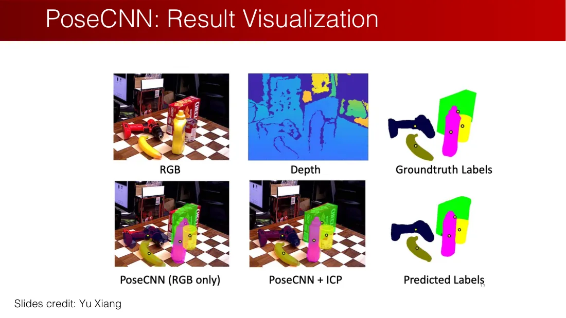
Lecture 05 · PDF p63
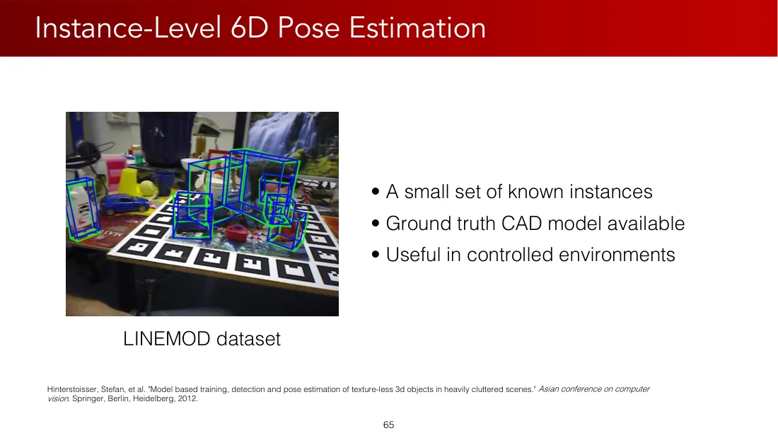
Lecture 05 · PDF p64
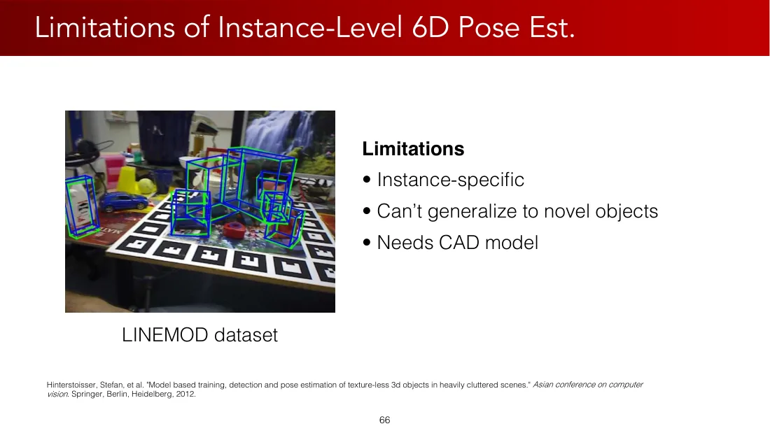
Lecture 05 · PDF p65
Lecture 05 · PDF p66
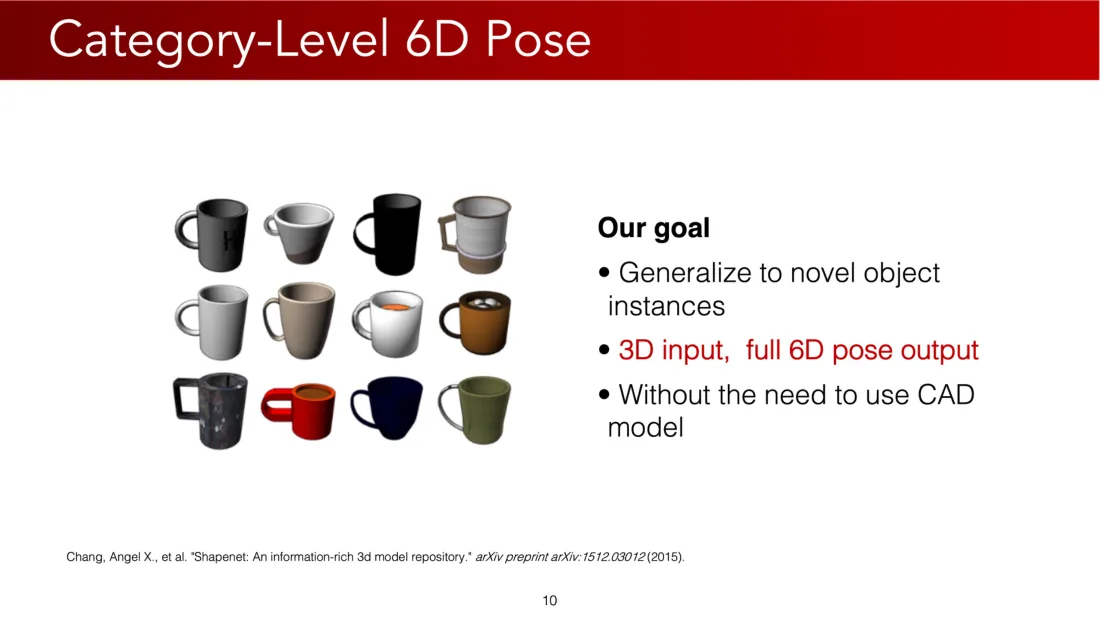
Lecture 05 · PDF p67
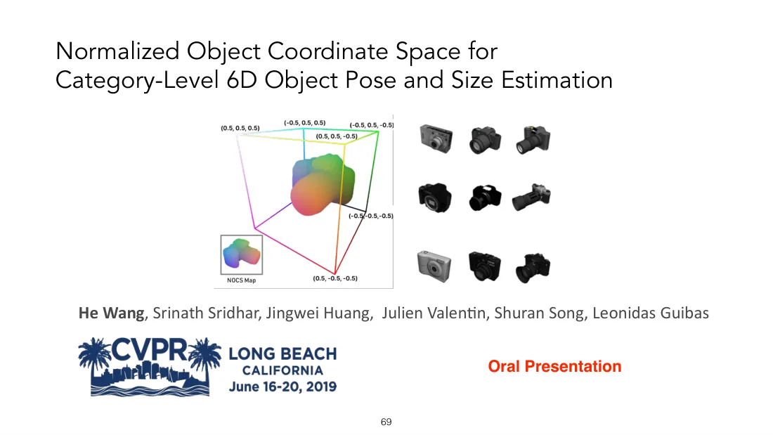
Lecture 05 · PDF p68
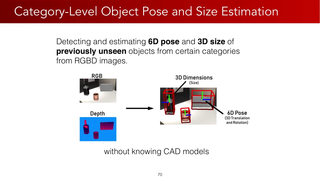
Lecture 05 · PDF p69
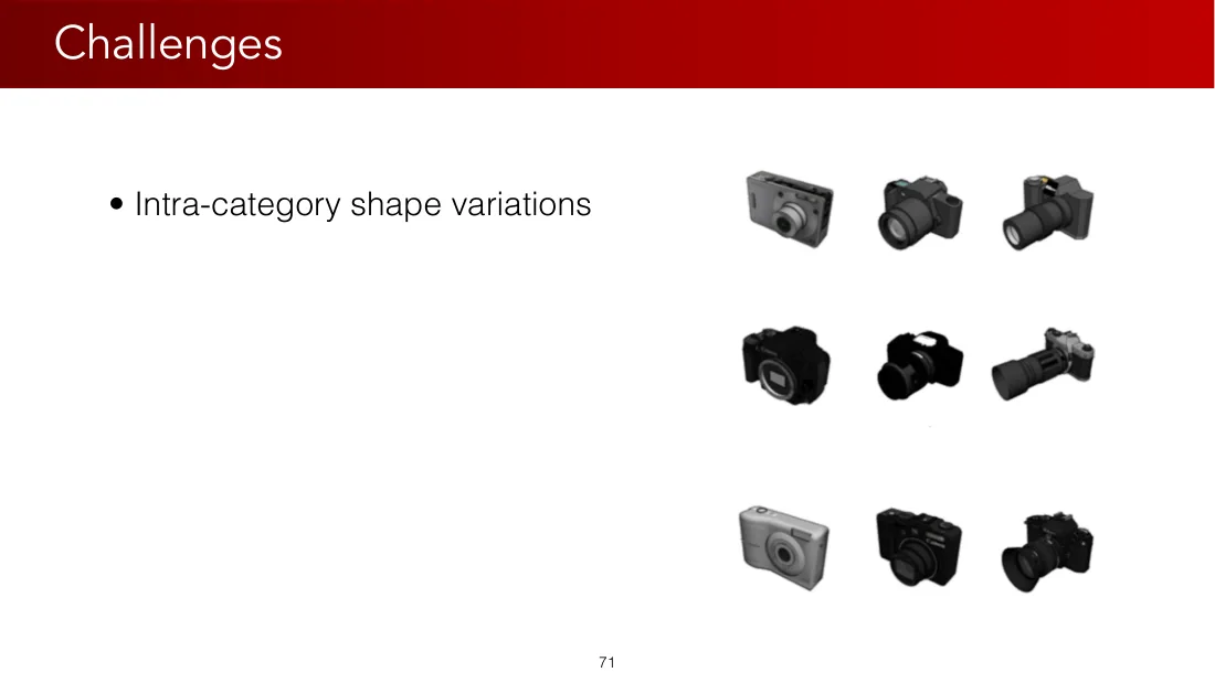
Lecture 05 · PDF p70
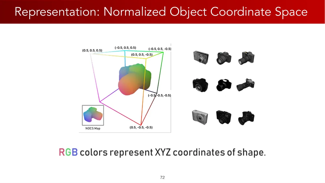
Lecture 05 · PDF p71