第4章 · 原课件与完整中文翻译
上方为英文原页,下方为对应的完整中文翻译,标题、正文、图内文字和公式按原页顺序排列。
页号按PDF顺序。原课件的历史日期、学期、课堂安排和研究结论按原文保留;相关概念与适用条件见教程正文。符号、代码、作者姓名及便于检索的专有名称保留原文。
Lecture 04 · 61页
Lecture 04 · PDF p1
Lecture 04 · PDF p2
Lecture 04 · PDF p3
Lecture 04 · PDF p4
Lecture 04 · PDF p5
Lecture 04 · PDF p6
Lecture 04 · PDF p7
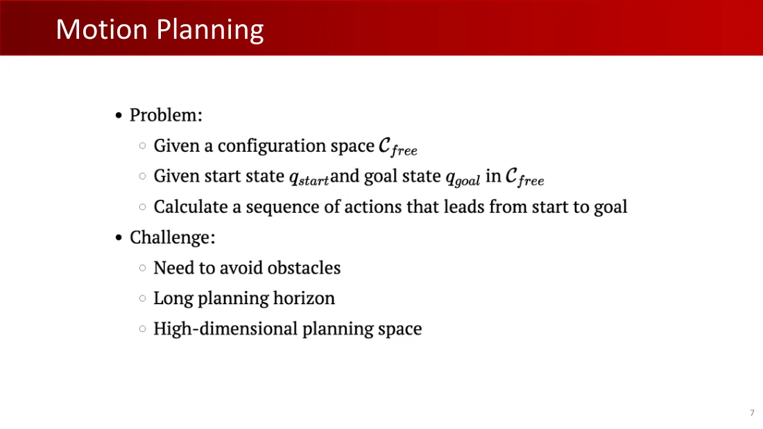
Lecture 04 · PDF p8
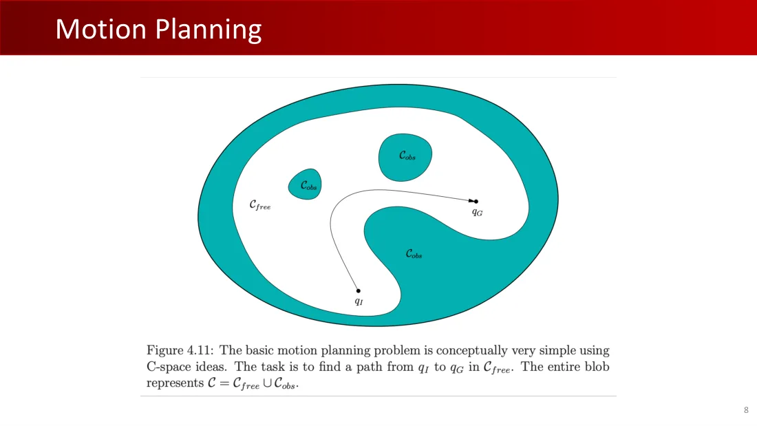
Lecture 04 · PDF p9
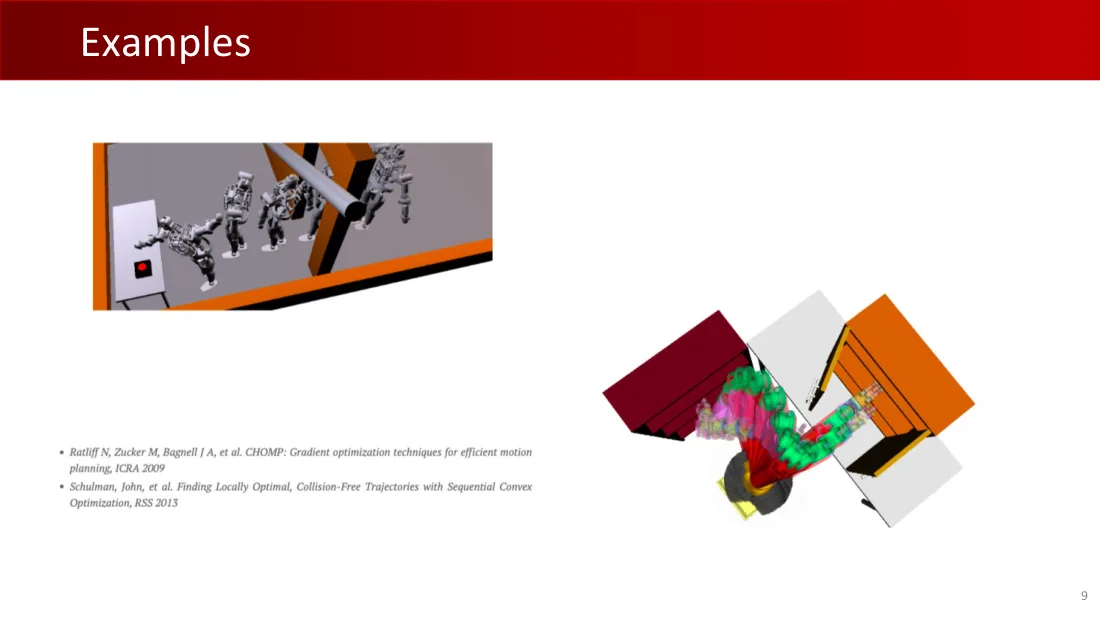
Lecture 04 · PDF p10
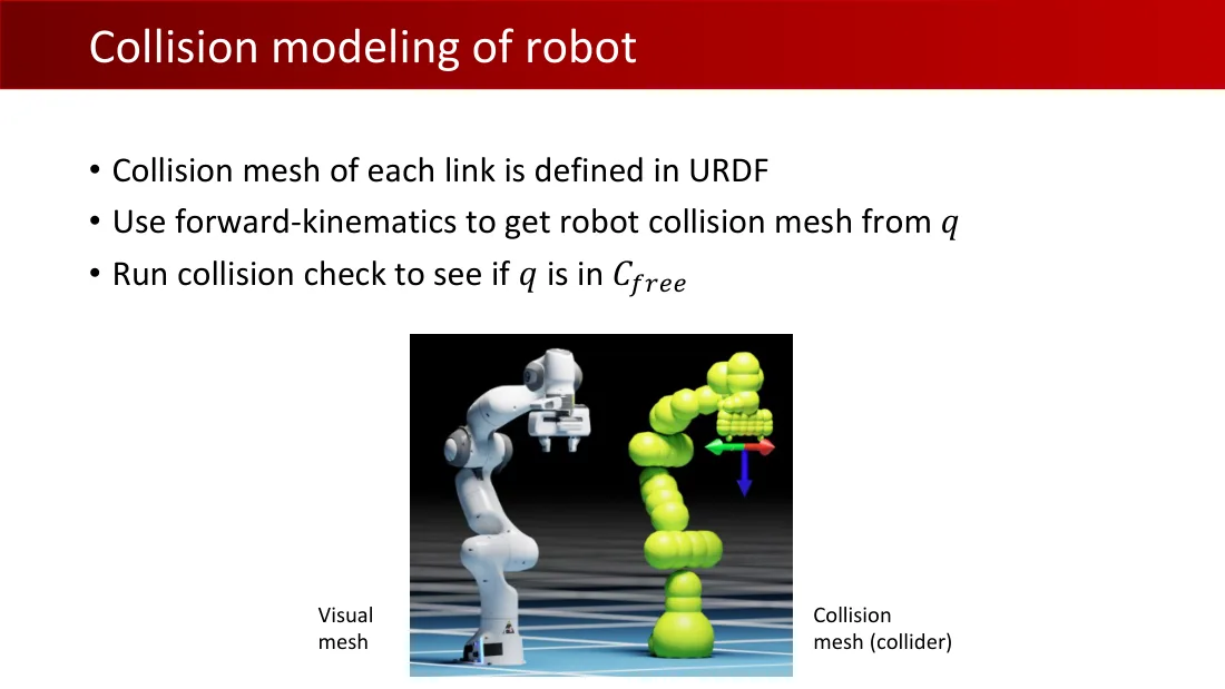
Lecture 04 · PDF p11
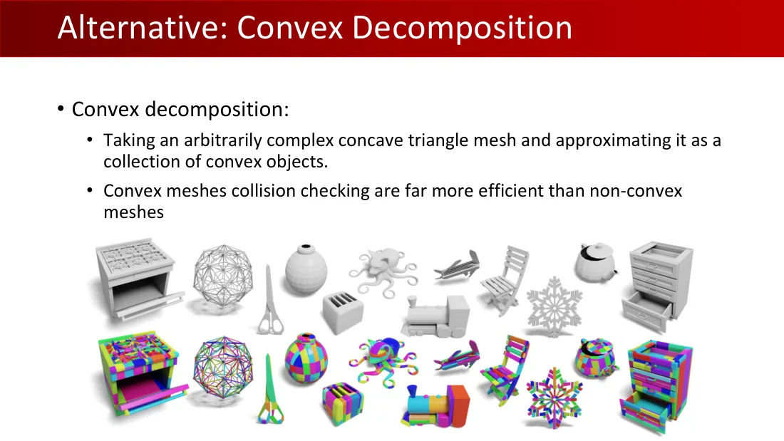
Lecture 04 · PDF p12
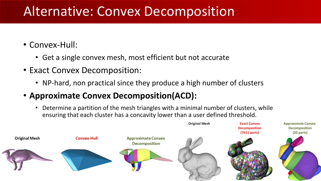
Lecture 04 · PDF p13
Lecture 04 · PDF p14
Lecture 04 · PDF p15
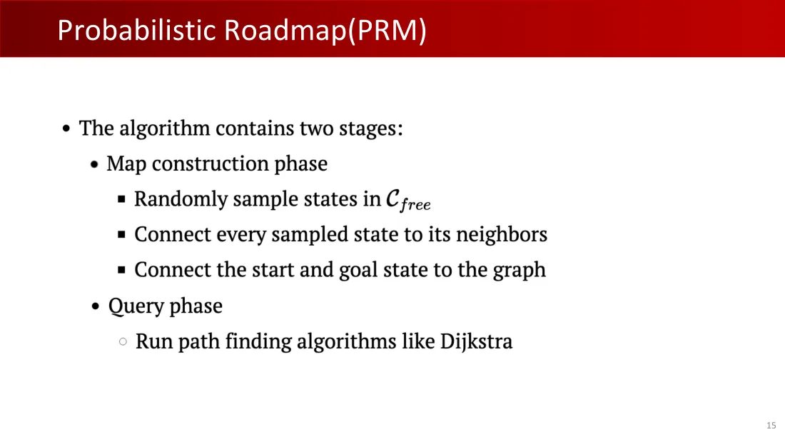
Lecture 04 · PDF p16
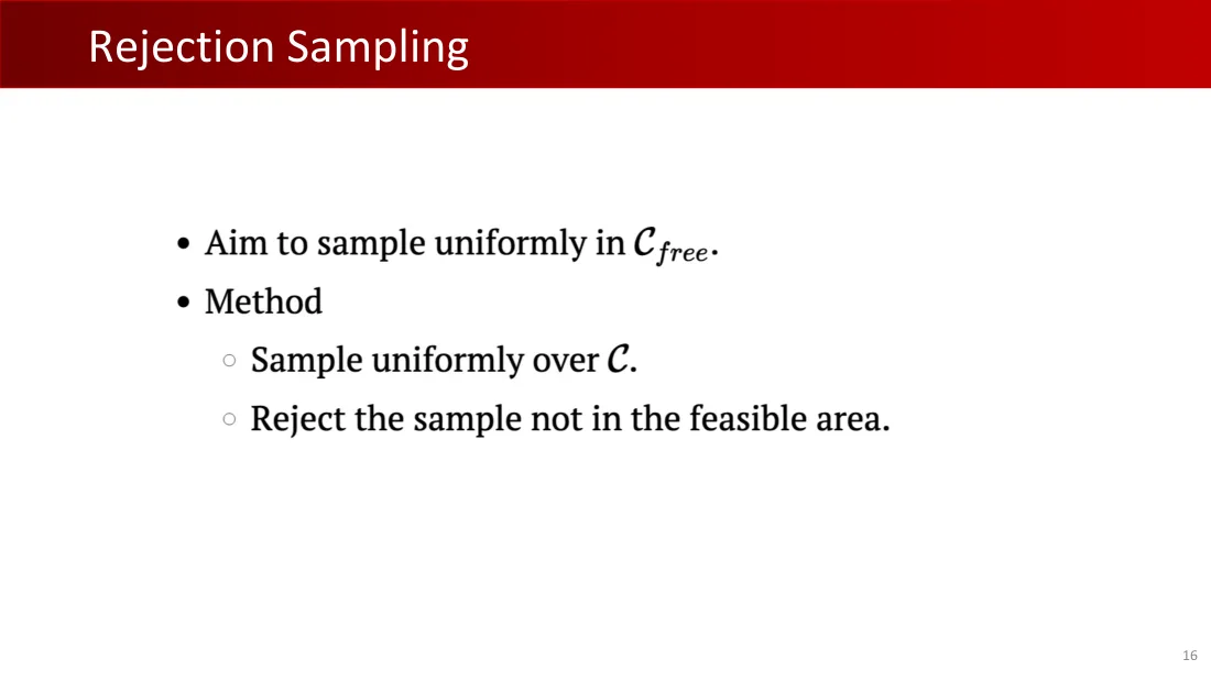
Lecture 04 · PDF p17
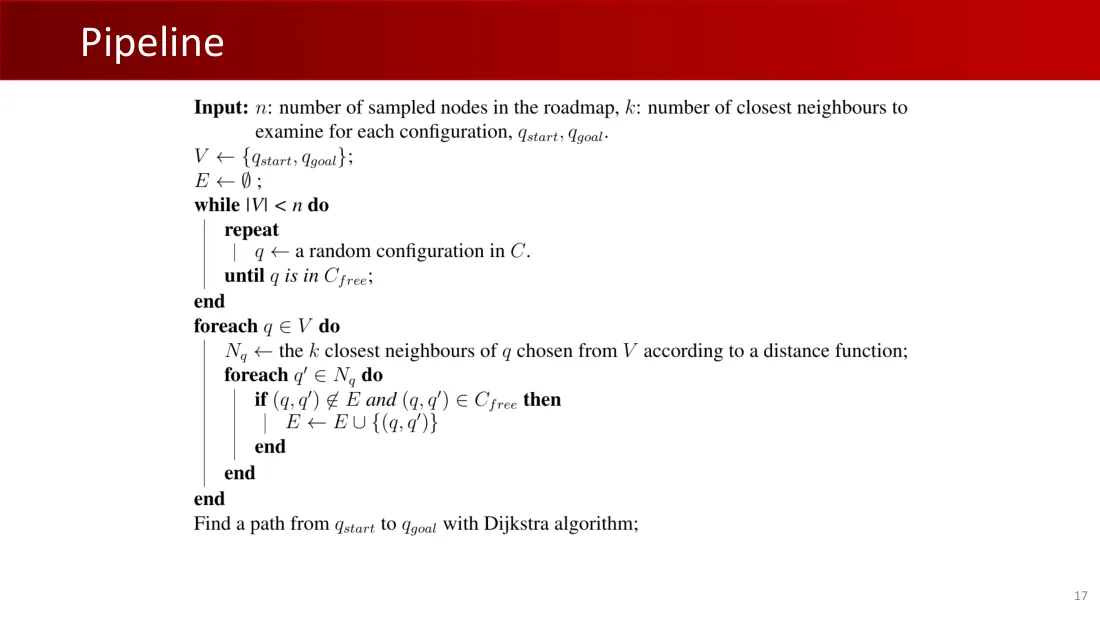
输入:n为路图中的采样节点数,k为每个配置需检查的最近邻数,\(q_{\mathrm{start}}\)、\(q_{\mathrm{goal}}\)。
\(V\leftarrow\{q_{\mathrm{start}},q_{\mathrm{goal}}\};\quad E\leftarrow\varnothing\)。
- 当\(|V|
- 对每个\(q\in V\):
- \(N_q\)←根据距离函数,从V中选取q的k个最近邻。
- 对每个\(q^{\prime}\in N_q\):若\((q,q^{\prime})\notin E\)且\((q,q^{\prime})\in C_{\mathrm{free}}\),则\(E\leftarrow E\cup\{(q,q^{\prime})\}\)。
- 对每个\(q\in V\):
使用Dijkstra算法寻找从\(q_{\mathrm{start}}\)到\(q_{\mathrm{goal}}\)的路径。
Lecture 04 · PDF p18
Lecture 04 · PDF p19
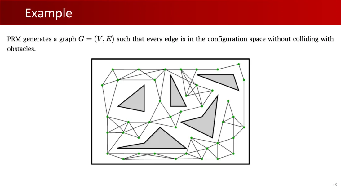
Lecture 04 · PDF p20
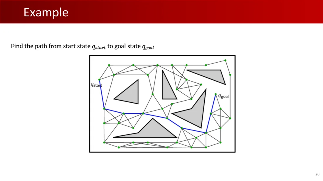
Lecture 04 · PDF p21
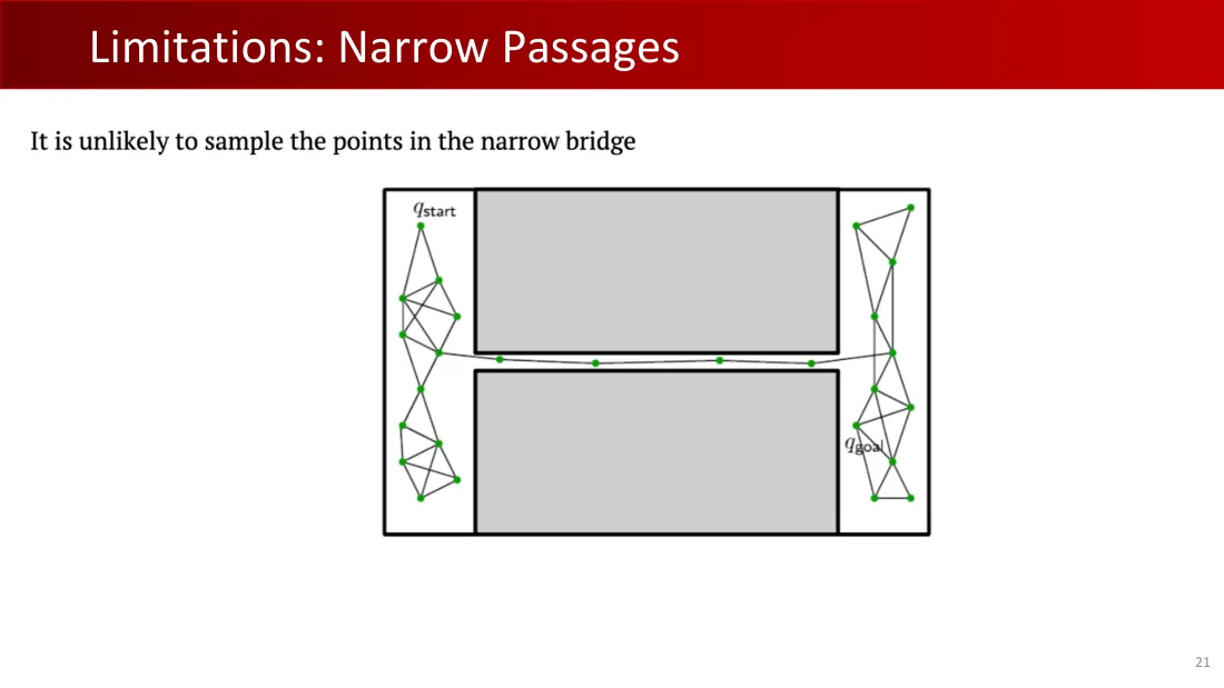
Lecture 04 · PDF p22
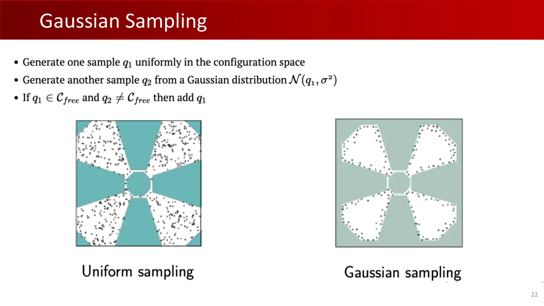
Lecture 04 · PDF p23
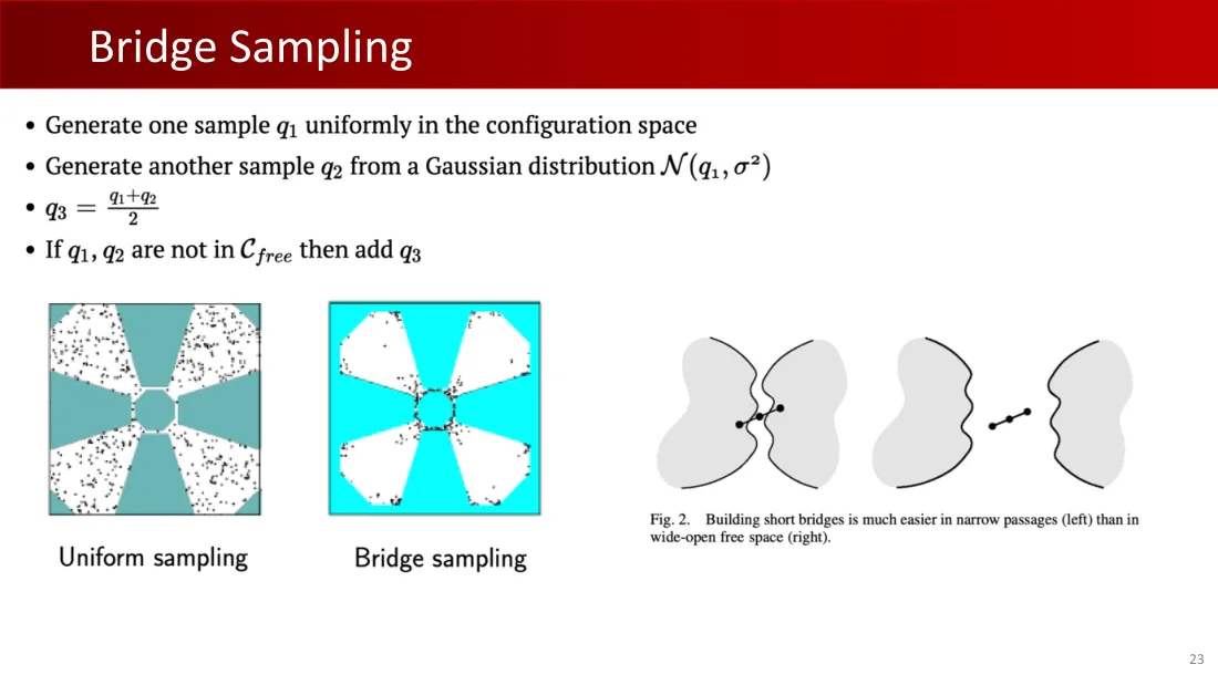
Lecture 04 · PDF p24
Lecture 04 · PDF p25
Lecture 04 · PDF p26
Lecture 04 · PDF p27
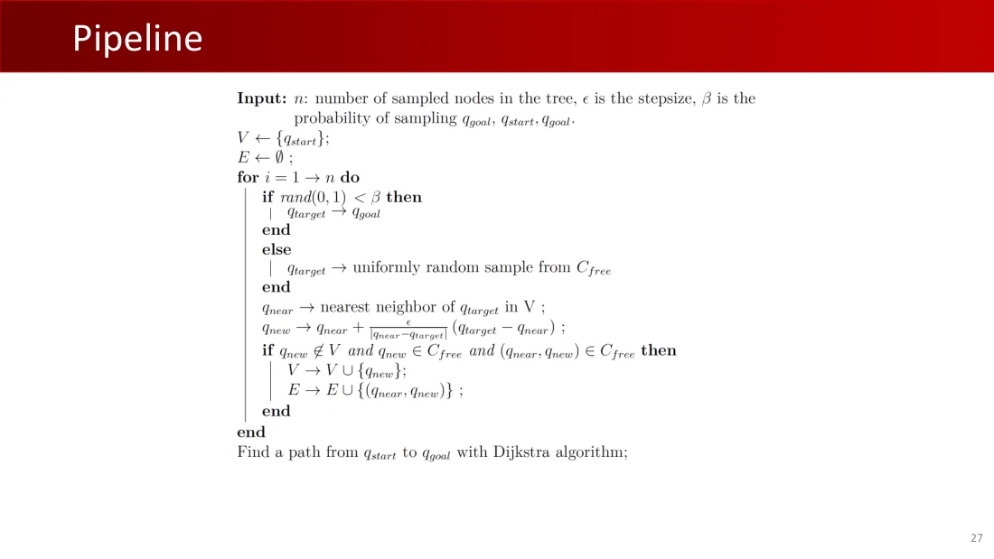
输入:n为树中的采样节点数,\(\varepsilon\)为步长,\(\beta\)为采样\(q_{\mathrm{goal}}\)的概率,\(q_{\mathrm{start}}\)、\(q_{\mathrm{goal}}\)。
\(V\leftarrow\{q_{\mathrm{start}}\};\quad E\leftarrow\varnothing\)。
- 对i=1至n:
- 若\(\operatorname{rand}(0,1)<\beta\),则\(q_{\mathrm{target}}\leftarrow q_{\mathrm{goal}}\);否则\(q_{\mathrm{target}}\)←从\(C_{\mathrm{free}}\)均匀随机采样。
- \(q_{\mathrm{near}}\)←V中\(q_{\mathrm{target}}\)的最近邻。
- \(q_{\mathrm{new}}\leftarrow q_{\mathrm{near}}+\varepsilon\frac{q_{\mathrm{target}}-q_{\mathrm{near}}}{|q_{\mathrm{near}}-q_{\mathrm{target}}|}\)。
- 若\(q_{\mathrm{new}}\notin V\)、\(q_{\mathrm{new}}\in C_{\mathrm{free}}\)且\((q_{\mathrm{near}},q_{\mathrm{new}})\in C_{\mathrm{free}}\),则\(V\leftarrow V\cup\{q_{\mathrm{new}}\}\),\(E\leftarrow E\cup\{(q_{\mathrm{near}},q_{\mathrm{new}})\}\)。
使用Dijkstra算法寻找从\(q_{\mathrm{start}}\)到\(q_{\mathrm{goal}}\)的路径。
Lecture 04 · PDF p28
Lecture 04 · PDF p29
Lecture 04 · PDF p30
RANDOM_CONFIG(\(q_{\mathrm{goal}}\)):随机配置
若\(\operatorname{rand}(0,1)<\beta\),返回\(q_{\mathrm{goal}}\);否则返回\(C_{\mathrm{free}}\)中的随机样本。
EXTEND(T,q):扩展
- \(q_{\mathrm{near}}\)←NEAREST_NEIGHBOR(T,q)。
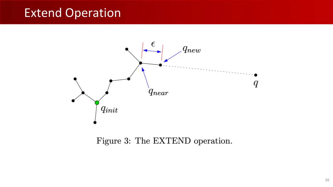
- 若\(|q_{\mathrm{near}}-q|<\varepsilon\),\(q_{\mathrm{new}}\leftarrow q\);否则\(q_{\mathrm{new}}\leftarrow q_{\mathrm{near}}+\varepsilon\frac{q-q_{\mathrm{near}}}{|q-q_{\mathrm{near}}|}\)。
- 若\(q_{\mathrm{new}}\in C_{\mathrm{free}}\)且\((q_{\mathrm{near}},q_{\mathrm{new}})\in C_{\mathrm{free}}\):T.add_vertex(\(q_{\mathrm{new}}\)),T.add_edge((\(q_{\mathrm{near}}\),\(q_{\mathrm{new}}\)));若\(q_{\mathrm{new}}=q\),返回Reached(到达),否则返回Advanced(前进)。
- 否则返回Trapped(受阻)。
CONNECT(T,q):连接
重复S←EXTEND(T,q),直到S≠Advanced;返回S。
RRT_CONNECT(\(q_{\mathrm{start}}\),\(q_{\mathrm{goal}}\))
- T_a.init(\(q_{\mathrm{start}}\)),T_b.init(\(q_{\mathrm{goal}}\))。
- 对k=1至K:q_rand←RANDOM_CONFIG(\(q_{\mathrm{goal}}\));若EXTEND(T_a,q_rand)≠Trapped且CONNECT(T_b,\(q_{\mathrm{new}}\))=Reached,返回PATH(T_a,T_b);交换\(q_{\mathrm{start}}\)与\(q_{\mathrm{goal}}\),交换T_a与T_b。
- 返回Failure(失败)。
Lecture 04 · PDF p31
Lecture 04 · PDF p32
Lecture 04 · PDF p33
Lecture 04 · PDF p34
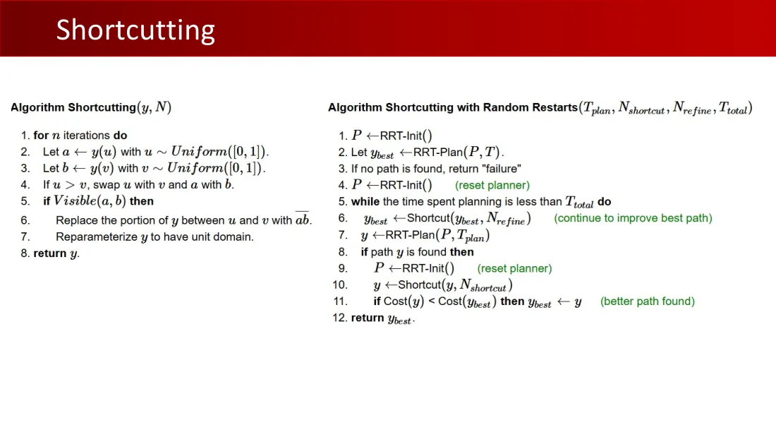
算法:Shortcutting(y,N)
- 执行n次迭代。
- 令\(a\leftarrow y(u)\),其中\(u\sim\operatorname{Uniform}([0,1])\)。
- 令\(b\leftarrow y(v)\),其中\(v\sim\operatorname{Uniform}([0,1])\)。
- 若\(u>v\),交换u、v,同时交换a、b。
- 若Visible(a,b),则用线段ab替换y中u至v的部分。
- 重新参数化y,使定义域为单位区间。
- 返回y。
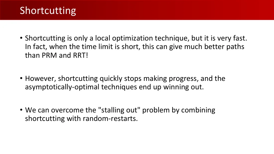
算法:带随机重启的捷径化(T_plan,N_shortcut,N_refine,T_total)
- P←RRT-Init()。
- y_best←RRT-Plan(P,T)。
- 若没有找到路径,返回“失败”。
- P←RRT-Init()(重置规划器)。
- 当规划耗时小于T_total:y_best←Shortcut(y_best,N_refine)(继续改进最佳路径);y←RRT-Plan(P,T_plan)。
- 若找到路径y:P←RRT-Init()(重置规划器);y←Shortcut(y,N_shortcut);若Cost(y)<Cost(y_best),则y_best←y(找到更好的路径)。
- 返回y_best。
Lecture 04 · PDF p35
Lecture 04 · PDF p36
Lecture 04 · PDF p37
Lecture 04 · PDF p38
Lecture 04 · PDF p39
Lecture 04 · PDF p40
Lecture 04 · PDF p41
Lecture 04 · PDF p42
Lecture 04 · PDF p43
Lecture 04 · PDF p44
Lecture 04 · PDF p45
Lecture 04 · PDF p46
Lecture 04 · PDF p47
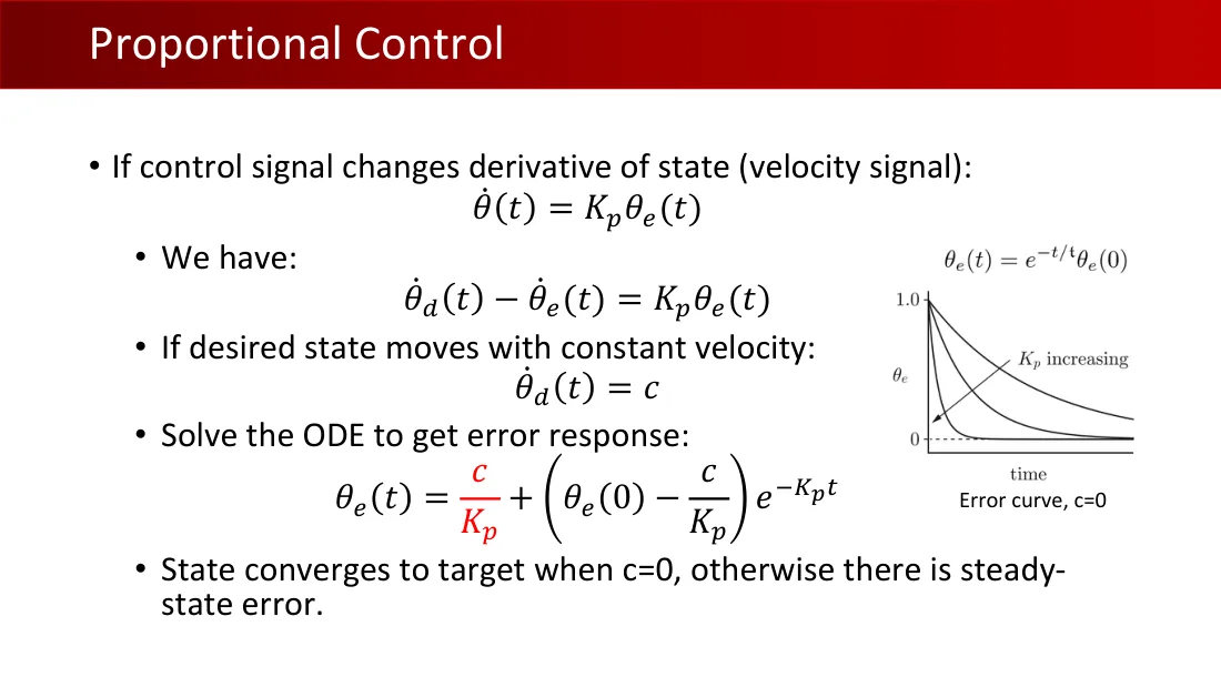
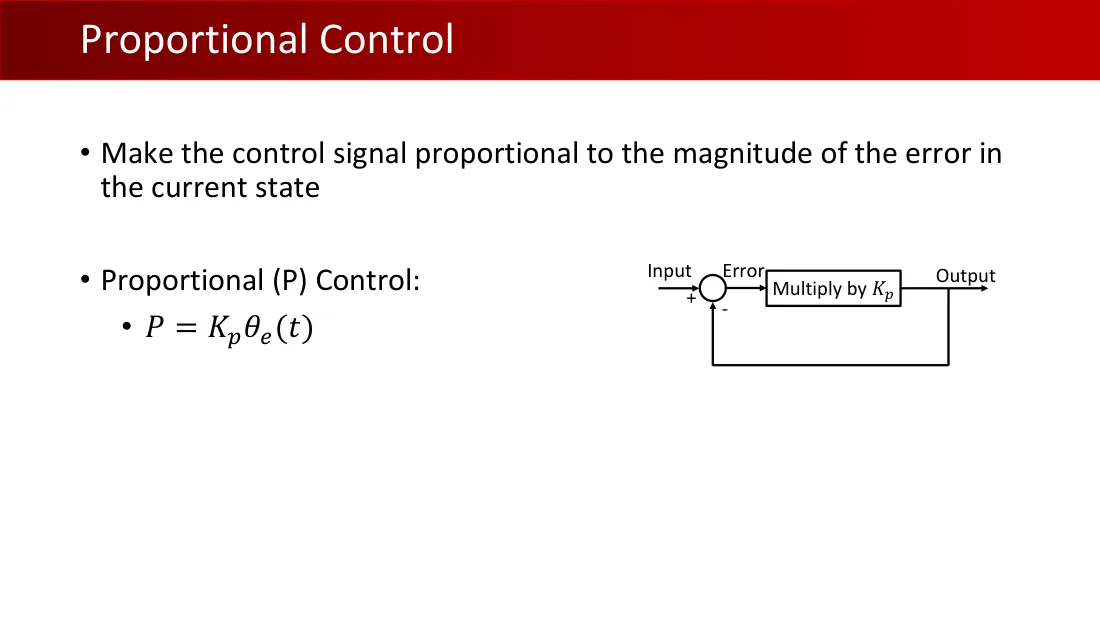
- 若控制信号改变状态的一阶导数(速度信号):\(\dot\theta(t)=K_p\theta_e(t)\)。
- 有:\(\dot\theta_d(t)-\dot\theta_e(t)=K_p\theta_e(t)\)。
- 若期望状态以恒定速度移动:\(\dot\theta_d(t)=c\)。
- 求解常微分方程得到误差响应:\(\theta_e(t)=\frac{c}{K_p}+\left(\theta_e(0)-\frac{c}{K_p}\right)e^{-K_pt}\)。
- c=0时状态收敛至目标,否则存在稳态误差。
\(\theta_e(t)=e^{-t/\tau}\theta_e(0)\);\(K_p\)增大;时间;误差曲线,c=0。
Lecture 04 · PDF p48
Lecture 04 · PDF p49
Lecture 04 · PDF p50
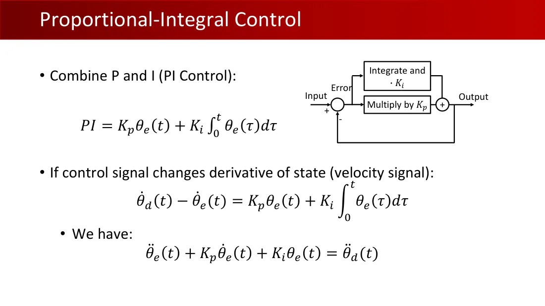
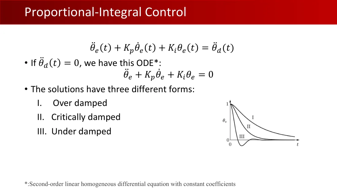
- 将P与I结合(PI控制):\(\mathrm{PI}=K_p\theta_e(t)+K_i\int_0^t\theta_e(\tau)\,d\tau\)。
- 若控制信号改变状态的一阶导数(速度信号):\(\dot\theta_d(t)-\dot\theta_e(t)=K_p\theta_e(t)+K_i\int_0^t\theta_e(\tau)\,d\tau\)。
- 有:\(\ddot\theta_e(t)+K_p\dot\theta_e(t)+K_i\theta_e(t)=\ddot\theta_d(t)\)。
输入;误差;积分并乘以\(K_i\);乘以\(K_p\);输出。
Lecture 04 · PDF p51
Lecture 04 · PDF p52
Lecture 04 · PDF p53
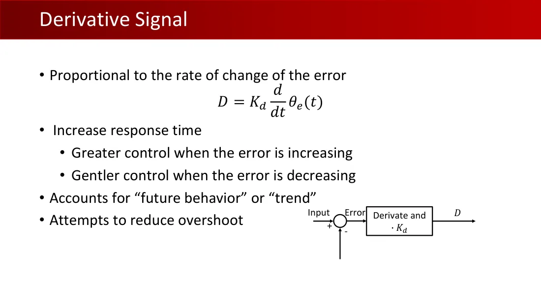
Lecture 04 · PDF p54
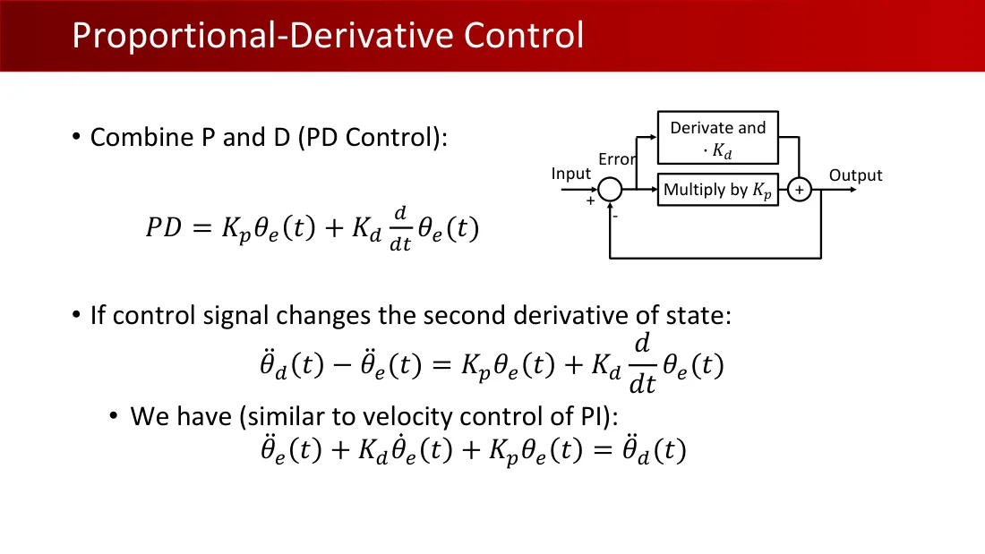
- 将P与D结合(PD控制):\(\mathrm{PD}=K_p\theta_e(t)+K_d\frac{d}{dt}\theta_e(t)\)。
- 若控制信号改变状态二阶导数:\(\ddot\theta_d(t)-\ddot\theta_e(t)=K_p\theta_e(t)+K_d\frac{d}{dt}\theta_e(t)\)。
- 有(类似PI的速度控制):\(\ddot\theta_e(t)+K_d\dot\theta_e(t)+K_p\theta_e(t)=\ddot\theta_d(t)\)。
输入;误差;求导并乘以\(K_d\);乘以\(K_p\);输出。
Lecture 04 · PDF p55
Lecture 04 · PDF p56
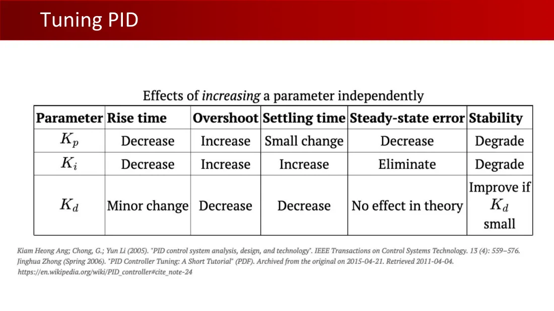
独立增大一个参数的影响
| 参数 | 上升时间 | 超调 | 调节时间 | 稳态误差 | 稳定性 |
|---|---|---|---|---|---|
| \(K_p\) | 减小 | 增大 | 小变化 | 减小 | 变差 |
| \(K_i\) | 减小 | 增大 | 增大 | 消除 | 变差 |
| \(K_d\) | 小变化 | 减小 | 减小 | 理论上无影响 | \(K_d\)小时改善 |
Kiam Heong Ang; Chong, G.; Yun Li(2005)。《PID控制系统分析、设计与技术》。IEEE Transactions on Control Systems Technology,13(4):559–576。
Jinghua Zhong(2006年春)。《PID控制器调参:简短教程》(PDF)。2015-04-21存档,2011-04-04查阅。
https://en.wikipedia.org/wiki/PID_controller#cite_note-24
Lecture 04 · PDF p57
Lecture 04 · PDF p58
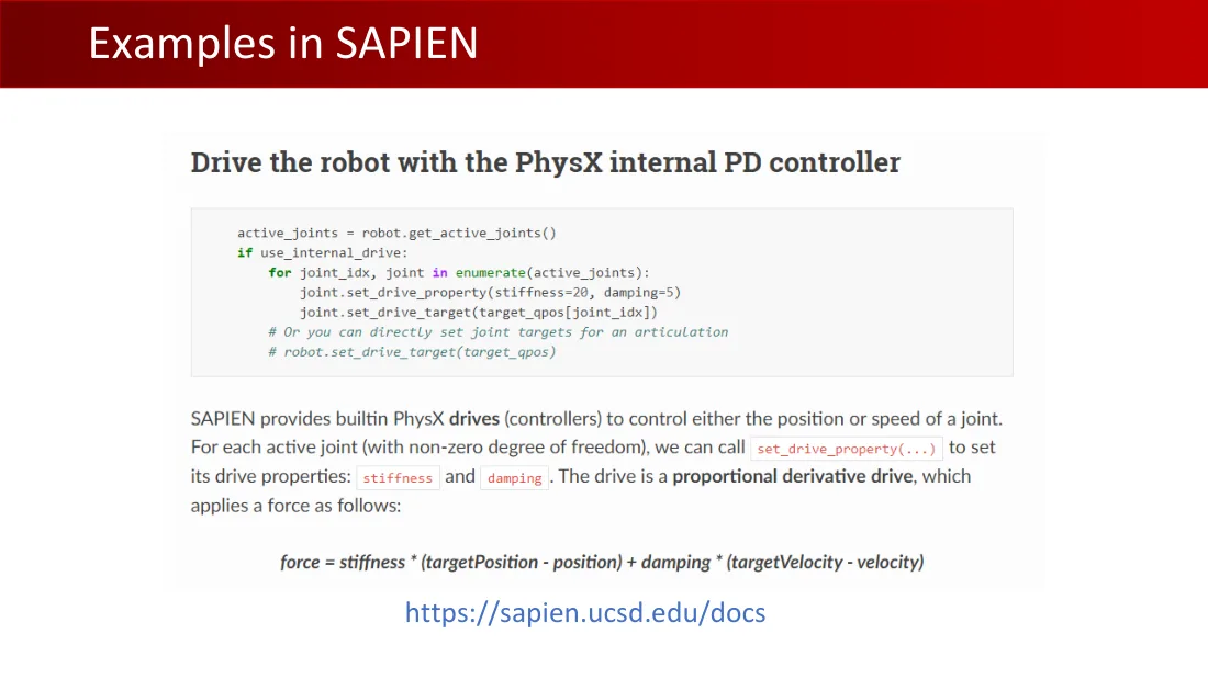
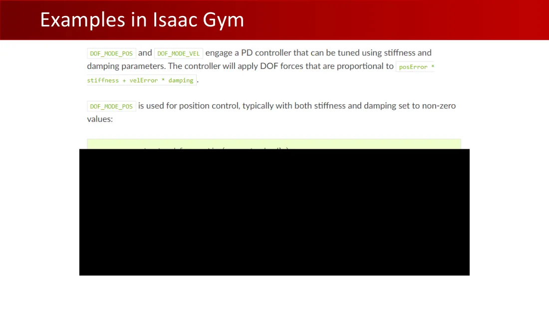
使用PhysX内部PD控制器驱动机器人
active_joints = robot.get_active_joints()
if use_internal_drive:
for joint_idx, joint in enumerate(active_joints):
joint.set_drive_property(stiffness=20, damping=5)
joint.set_drive_target(target_qpos[joint_idx])
# 或者,直接为整个关节结构设置关节目标
# robot.set_drive_target(target_qpos)
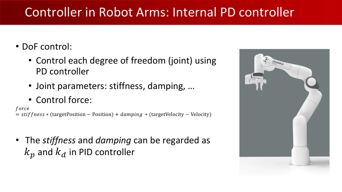
SAPIEN提供内置PhysX驱动(控制器),以控制关节的位置或速度。对每个活动关节(自由度非零),可调用set_drive_property(...)设置驱动属性stiffness(刚度)和damping(阻尼)。驱动采用比例微分形式,施加的力如下:
\(\mathrm{force}=\mathrm{stiffness}\cdot(\mathrm{targetPosition}-\mathrm{position})+\mathrm{damping}\cdot(\mathrm{targetVelocity}-\mathrm{velocity})\)
https://sapien.ucsd.edu/docs
Lecture 04 · PDF p59
Lecture 04 · PDF p60
Lecture 04 · PDF p61